
Mastering Decision Trees
Table of Contents
- Introduction
- Purity Measures
- Splitting Criteria & Gain
- Algorithms for Constructing a Decision Tree
- Pruning Methods to Avoid Over-Fitting
- Regression Trees
- Practical Implementation
- Model Evaluation
- Extensions & Variants
- Best Practices & Common Pitfalls
- Conclusion & Further Reading
1. Introduction
Welcome to this deep dive into Decision Trees, a fundamental and powerful algorithm in the machine learning toolkit. Whether you're new to ML or looking to solidify your understanding, this guide aims to provide a comprehensive overview, blending theory with practical insights.
1.1. What Is Classification?
At its core, classification is a type of supervised learning problem where the goal is to assign input data points to one of several predefined categories or classes. Think of it like sorting mail into different bins based on zip codes, or identifying emails as either "spam" or "not spam".
Formally, given a dataset , where each is a feature vector representing an instance and is its corresponding class label from a finite set of classes , the objective of a classification algorithm is to learn a mapping function . This function , often called a classifier or model, takes an unseen feature vector as input and predicts its class label .
Examples include:
- Image Recognition: Classifying images as containing a 'cat', 'dog', or 'bird'.
- Medical Diagnosis: Predicting whether a patient has a certain 'disease' or 'no disease' based on symptoms.
- Sentiment Analysis: Categorizing text reviews as 'positive', 'negative', or 'neutral'.
1.2. Why Decision Trees?
Among the myriad of classification algorithms, Decision Trees hold a special place for several compelling reasons:
- Interpretability: Decision Trees are often called "white box" models. The decision-making process mirrors human reasoning – a series of questions leading to a conclusion. This makes them relatively easy to understand, visualize, and explain, even to non-technical audiences.
- Minimal Data Preparation: They often require less data pre-processing compared to other methods. They don't strictly require data normalization or scaling and can inherently handle both numerical and categorical features (though some implementations might have specific requirements).
- Handling Non-linearity: Decision Trees can naturally capture non-linear relationships between features and the target variable without requiring complex transformations like polynomial features.
- Feature Importance: They implicitly perform a form of feature selection. The features used higher up in the tree are generally more influential in the classification process.
However, they are not without drawbacks (which we'll explore later), such as a tendency to overfit the training data.
1.3. Real-world Applications
Decision Trees and their ensemble variants (like Random Forests and Gradient Boosted Trees) are widely used across various domains:
- Finance: Credit scoring (predicting loan default risk), fraud detection.
- Healthcare: Disease diagnosis based on patient symptoms, predicting patient response to treatments.
- Marketing: Customer churn prediction, identifying customer segments for targeted campaigns.
- Manufacturing: Predictive maintenance (predicting machine failures), quality control.
- Biology: Classifying species based on observed characteristics.
Their intuitive structure makes them particularly useful in scenarios where understanding the why behind a prediction is as crucial as the prediction itself.
2. Purity Measures
The fundamental idea behind building a decision tree is to recursively split the dataset into subsets that are increasingly "pure" in terms of their class labels. But how do we quantify this purity? We need a mathematical measure to evaluate how mixed or homogeneous the class labels are within a node (a subset of data). A perfectly pure node contains samples belonging to only one class.
2.1. Node Purity (Definition)
A node in a decision tree represents a subset of the training data. Node purity refers to the degree to which all data points within that node belong to the same class.
- A pure node is one where all samples belong to a single class. This is the ideal state for a leaf node in the tree.
- An impure node contains a mix of samples from different classes.
The goal of the splitting process is to find splits (based on feature values) that result in child nodes that are, on average, purer than the parent node. Several metrics can be used to measure impurity (or its inverse, purity). The most common ones are Entropy, Gini Index, and Classification Error.
2.2. Entropy
Originating from information theory, Entropy measures the amount of uncertainty or randomness in a set of data. In the context of decision trees, it quantifies the impurity of a node .
2.2.1. Formula
Let be a set of training examples at a particular node. Let be the number of distinct classes. Let be the proportion (relative frequency) of examples in that belong to class . The entropy is defined as:
Note: By convention, . The logarithm is usually base 2 (), meaning entropy is measured in "bits". However, other bases (like the natural logarithm) can also be used, simply scaling the result.
2.2.2. Properties of Entropy
- Maximum Impurity: Entropy is maximized when the classes are equally distributed. For a two-class problem (), entropy is 1 when . Maximum entropy occurs at .
- Minimum Impurity (Purity): Entropy is 0 when the node is perfectly pure, i.e., all samples belong to a single class ( for some , and for all ).
- Range: For classes, .
Example: Consider a node with 10 samples: 6 'Positive' (+) and 4 'Negative' (-). bits. This value is close to the maximum (1 bit for k=2), indicating significant impurity.
2.3. Gini Index (or Gini Impurity)
The Gini Index is another popular measure of node impurity. It represents the probability of misclassifying a randomly chosen element from the set if it were randomly labeled according to the distribution of labels in .
2.3.1. Formula
Using the same notation as for entropy ( is the proportion of class in set ), the Gini Index is defined as:
Alternatively, it can be expressed as the sum of probabilities of picking an item of class times the probability of misclassifying it: .
2.3.2. Properties and Relation to Misclassification Error
- Maximum Impurity: Gini Index is maximized when classes are evenly distributed. For classes, this maximum is . For two classes, the maximum is .
- Minimum Impurity (Purity): Gini Index is 0 when the node is perfectly pure ( for some ).
- Range: .
- Interpretation: It can be seen as the expected error rate if we classify examples based on the empirical distribution in the node. It measures the "variance" across classes.
Example: Using the same node (6+, 4-): ,
2.4. Classification Error Rate
This is the simplest impurity measure. It directly calculates the probability of making an error if we assign every instance in the node to the most frequent class.
2.4.1. Formula
The Classification Error is defined as:
- Maximum Impurity: Like the Gini Index, the maximum occurs when classes are evenly distributed, reaching . For two classes, the maximum is .
- Minimum Impurity (Purity): Error rate is 0 when the node is pure ().
- Range: .
Example: Using the same node (6+, 4-): ,
2.5. Comparing Purity Metrics
- Sensitivity: Entropy and Gini Index are more sensitive to changes in the node's probability distribution than the Classification Error rate. For example, if we have a node with proportions (0.49, 0.51) and another with (0.1, 0.9), the Classification Error is almost the same (0.49 vs 0.1), while Entropy and Gini will show a much larger difference, correctly indicating the second node is significantly purer. Because of this lack of sensitivity, Classification Error is rarely used directly for selecting splits during tree growth, though it might be used for pruning.
- Computational Cost: Gini Index is often slightly faster to compute as it avoids the logarithm calculation present in Entropy. This is one reason it's the default criterion in many libraries like scikit-learn.
- Resulting Trees: Although their mathematical formulations differ, Gini Index and Entropy often produce very similar trees in practice. Entropy tends to favor slightly more balanced splits, while Gini can sometimes isolate smaller, purer nodes more quickly.
In the next section, we'll discuss how these purity measures are used to evaluate potential splits using concepts like Information Gain.
3. Splitting Criteria & Gain
Now that we understand how to measure the impurity of a node (using Entropy, Gini Index, or Classification Error), the next step in building a decision tree is to determine the "best" attribute and split point to partition the data. The "best" split is the one that results in the most homogeneous (purest) child nodes, or equivalently, the one that reduces impurity the most. This reduction in impurity is often referred to as "Gain".
3.1. Information Gain
Information Gain (IG) is the most common splitting criterion when using Entropy as the impurity measure. It quantifies the expected reduction in entropy achieved by splitting the dataset based on an attribute . The attribute that provides the maximum Information Gain is chosen for the split.
3.1.1. Formula
Let be a set of training examples at a parent node. Let be an attribute with distinct values (or possible outcomes of a test on , e.g., and for a continuous attribute). Splitting on attribute partitions into subsets , where is the subset of for which attribute has value .
The Information Gain of attribute for set is defined as:
Where:
- is the entropy of the parent node .
- is the set of all possible values of attribute .
- is the number of examples in the subset .
- is the total number of examples in .
- is the entropy of the subset .
The term represents the weighted average entropy of the child nodes after splitting on attribute . Thus, Information Gain is simply the entropy of the parent minus the weighted average entropy of the children. We want to maximize this gain.
How it works for different attribute types:
- Categorical Attributes: If an attribute is categorical (e.g., 'Color' with values 'Red', 'Green', 'Blue'), the sum is over these distinct values. Each value typically forms a branch.
- Continuous Attributes: For a continuous attribute (e.g., 'Temperature'), a split point (threshold) must be determined. Common practice is to sort the unique values of the attribute present in the dataset and consider midpoints between successive sorted values as potential split points. For each potential split point , the data is divided into two subsets ( and ), and the Information Gain is calculated. The split point yielding the highest IG is chosen for that attribute. The attribute (and its best split point) with the overall highest IG is then selected for the node.
Limitation of Information Gain: Information Gain has a bias towards attributes with a large number of distinct values. For example, an attribute like 'CustomerID' would have a very high IG because it would split the data into many pure (or near-pure) nodes, each containing only one customer. However, such a split is not generalizable and leads to overfitting. This is where Gain Ratio comes in.
3.2. Gain Ratio
To address the bias of Information Gain towards attributes with many values, Gain Ratio was introduced (most notably by the C4.5 algorithm). It normalizes the Information Gain by the "Split Information" or "Intrinsic Information" of the attribute itself.
The Split Information (or Intrinsic Information), denoted or , measures the entropy of the distribution of instances into branches created by attribute :
This term represents the potential information generated by splitting into subsets. It's high for attributes that split the data into many small, uniformly sized partitions and low for attributes that create few, imbalanced partitions.
The Gain Ratio is then defined as:
By dividing by , Gain Ratio penalizes attributes that create many small branches, such as ID codes.
Considerations for Gain Ratio:
- If is very small (close to 0), for example, if one branch contains almost all samples, Gain Ratio can become unstable or excessively large. Implementations (like C4.5) often have heuristics to handle this, e.g., by first computing the IG for all attributes and then, among those with at least average IG, selecting the one with the highest Gain Ratio.
3.3. Gini Gain (or Impurity Reduction)
When using the Gini Index as the impurity measure, the equivalent of Information Gain is often referred to as Gini Gain or simply the reduction in Gini impurity. The principle is identical: calculate the Gini impurity of the parent node and subtract the weighted average Gini impurity of the child nodes.
Let be the Gini Index of the parent node . If attribute splits into subsets , the Gini Gain is:
The attribute and split point that maximize the Gini Gain are chosen for the split.
Why Gini Gain is popular (used in CART):
- Computational Efficiency: As mentioned earlier, Gini Index doesn't require logarithm calculations, making Gini Gain slightly faster to compute than Information Gain.
- Less Biased (compared to IG alone): While Gini Gain can still be somewhat biased towards multi-valued attributes, the effect is generally less pronounced than with Information Gain. It doesn't require an explicit normalization like Gain Ratio.
- Focus on Binary Splits: The CART algorithm, which uses Gini Gain, always produces binary trees. For categorical attributes with multiple values, it finds the best binary partition of these values (e.g., if is , it might test vs. ).
Choosing the right splitting criterion depends on the specific algorithm (ID3 uses Information Gain, C4.5 uses Gain Ratio, CART uses Gini Gain) and the characteristics of the data. In practice, both Gini Gain and Gain Ratio are robust and widely used.
4. Algorithms for Constructing a Decision Tree
Several algorithms have been developed to build decision trees. Most of them follow a greedy, top-down, recursive partitioning strategy. This means they start with the entire dataset at the root and, at each step, select the best attribute and split point to divide the current dataset into more homogeneous subsets. This process is repeated for each new subset (node) until a stopping criterion is met.
The primary differences between these algorithms lie in:
- The splitting criterion used (e.g., Information Gain, Gain Ratio, Gini Index).
- The types of attributes they can handle (categorical, numerical).
- How they handle missing values.
- The pruning methods they employ (or if they employ them during the growth phase).
Let's look at some of the most influential decision tree algorithms.
4.1. ID3 (Iterative Dichotomiser 3)
Developed by Ross Quinlan in the early 1980s, ID3 is one of the earliest and simplest decision tree algorithms.
- Splitting Criterion: Uses Information Gain (based on Entropy). At each node, it selects the attribute with the highest Information Gain to split the data.
- Attribute Types: Primarily designed for categorical attributes. It can be adapted for numerical attributes by discretizing them first (i.e., converting them into categorical ranges), but this is not its native strength.
- Tree Structure: Can produce multi-way splits (a branch for each distinct value of the chosen categorical attribute). This can lead to very bushy trees, especially with attributes having many unique values.
- Missing Values: Does not have a sophisticated built-in mechanism for handling missing values. Typically, instances with missing values for the selected attribute are either ignored or imputed.
- Pruning: Does not include a pruning step. It tends to grow the tree until all leaf nodes are pure or no more attributes can be used, making it very prone to overfitting the training data.
- Output: Generates a decision tree.
Key Idea: Greedily choose the attribute that provides the most information about the class labels at each step.
4.2. C4.5
C4.5 is the successor to ID3, also developed by Ross Quinlan, and addresses several of ID3's shortcomings.
- Splitting Criterion: Uses Gain Ratio (Information Gain normalized by Split Information). This helps to mitigate the bias of Information Gain towards attributes with many distinct values.
- Attribute Types: Natively handles both categorical and continuous (numerical) attributes.
- For continuous attributes, C4.5 finds an optimal threshold to split the data into two subsets (e.g., A ≤ threshold and A > threshold) by maximizing Gain Ratio.
- Tree Structure: Can produce multi-way splits for categorical attributes and binary splits for continuous attributes.
- Missing Values: Has a more sophisticated way of handling missing values. When calculating gain, it distributes instances with missing values proportionally among the outcomes of a potential split based on the distribution of other instances. During classification, if an instance encounters a split on an attribute for which it has a missing value, it can be fractionally passed down all branches according to the training data proportions, and the results are combined.
- Pruning: Includes a post-pruning step (error-based pruning) after the tree is fully grown. It converts the tree into a set of rules, prunes each rule by removing conditions if accuracy improves, and then reassembles the rules into a tree. This helps to improve generalization and reduce overfitting.
- Output: Generates a decision tree or a set of classification rules.
Key Improvements over ID3: Handling continuous attributes, using Gain Ratio, and incorporating a pruning mechanism.
4.3. CART (Classification and Regression Trees)
Developed by Leo Breiman, Jerome Friedman, Richard Olshen, and Charles Stone around the same time as ID3/C4.5, CART is another influential algorithm.
- Splitting Criterion:
- For Classification Trees: Uses Gini Index as the impurity measure and selects splits that maximize Gini Gain (reduction in Gini impurity).
- For Regression Trees: Uses measures like Mean Squared Error (MSE) or Least Absolute Deviation (LAD) to find splits that minimize the variance or error in the target variable within the child nodes.
- Attribute Types: Handles both categorical and continuous attributes.
- Tree Structure: Always produces binary trees.
- For categorical attributes with more than two values, CART evaluates all possible binary partitions of the values (e.g., vs. if values are A,B,C) and selects the one that maximizes Gini Gain.
- For continuous attributes, it finds the optimal threshold for a binary split.
- Missing Values: Has various methods for handling missing values, including "surrogate splits." If the best attribute for a split is missing for an instance, CART can use another "surrogate" attribute (whose split closely mimics the primary split) to route the instance.
- Pruning: Employs a sophisticated cost-complexity pruning (also known as weakest link pruning) method. It grows a large tree first and then prunes it back based on a cost-complexity parameter () that balances the tree's misclassification rate against its size. Cross-validation is typically used to find the optimal .
- Output: Generates binary classification or regression trees.
Key Features: Binary splits, Gini Index for classification, MSE/LAD for regression, and cost-complexity pruning.
4.4 Example: Building a Small Decision Tree (using ID3 with Information Gain)
Let's illustrate the tree-building process using the ID3 algorithm (Information Gain with Entropy) on the classic "Play Tennis" dataset.
Dataset (S):
| Outlook | Temp | Humidity | Windy | Play |
|---|---|---|---|---|
| Sunny | Hot | High | False | No |
| Sunny | Hot | High | True | No |
| Overcast | Hot | High | False | Yes |
| Rainy | Mild | High | False | Yes |
| Rainy | Cool | Normal | False | Yes |
| Rainy | Cool | Normal | True | No |
| Overcast | Cool | Normal | True | Yes |
| Sunny | Mild | High | False | No |
| Sunny | Cool | Normal | False | Yes |
| Rainy | Mild | Normal | False | Yes |
| Sunny | Mild | Normal | True | Yes |
| Overcast | Mild | High | True | Yes |
| Overcast | Hot | Normal | False | Yes |
| Rainy | Mild | High | True | No |
- Total instances: 14
- Play = Yes: 9 instances ()
- Play = No: 5 instances ()
Step 1: Calculate initial Entropy of the dataset S (Root Node) The entropy for a two-class problem is . bits.
Step 2: Calculate Information Gain for each attribute The Information Gain is . Attributes available: Outlook, Temp, Humidity, Windy. (Note: For this ID3 example, 'Temp' will be treated as categorical with values Hot, Mild, Cool.)
A. Attribute: Outlook
- Values: Sunny, Overcast, Rainy
- [2 Yes, 3 No]. .
- [4 Yes, 0 No]. .
- [3 Yes, 2 No]. .
- Weighted Average Entropy for Outlook:
- =
B. Attribute: Temp (treated as categorical: Hot, Mild, Cool)
- Values: Hot, Mild, Cool
- [2 Yes, 2 No]. .
- [4 Yes, 2 No]. .
- [3 Yes, 1 No]. .
- Weighted Average Entropy for Temp:
- =
C. Attribute: Humidity
- Values: High, Normal
- [3 Yes, 4 No]. .
- [6 Yes, 1 No]. .
- Weighted Average Entropy for Humidity:
- =
D. Attribute: Windy
- Values: False, True
- [6 Yes, 2 No]. .
- [3 Yes, 3 No]. .
- Weighted Average Entropy for Windy:
- =
Step 3: Select the attribute with the highest Information Gain
Outlook has the highest Information Gain (0.246). So, Outlook becomes the root node.
Step 4: Create branches for each value of Outlook and recursively build subtrees
-
Branch 1: Outlook = Sunny
- Dataset (5 instances): [2 Yes, 3 No]. Attributes remaining: Temp, Humidity, Windy.
- (calculated earlier)
- Calculate IG for Temp, Humidity, Windy on :
- IG(, Temp) =
- Hot (Sunny): [0Y, 2N] ->
- Mild (Sunny): [1Y, 1N] ->
- Cool (Sunny): [1Y, 0N] ->
- IG(, Temp) =
- IG(, Humidity):
- High (Sunny): 3 inst. [0Y, 3N] ->
- Normal (Sunny): 2 inst. [2Y, 0N] ->
- IG(, Humidity) = (Highest)
- IG(, Windy):
- False (Sunny): 3 inst. [1Y, 2N] ->
- True (Sunny): 2 inst. [1Y, 1N] ->
- IG(, Windy) =
- IG(, Temp) =
- Humidity is chosen for the split under Outlook=Sunny.
- Outlook=Sunny, Humidity=High (3 instances: [0 Yes, 3 No]) -> Leaf Node: Play = No (Pure)
- Outlook=Sunny, Humidity=Normal (2 instances: [2 Yes, 0 No]) -> Leaf Node: Play = Yes (Pure)
-
Branch 2: Outlook = Overcast
- Dataset (4 instances): [4 Yes, 0 No].
- This node is pure (all 'Yes'). -> Leaf Node: Play = Yes
-
Branch 3: Outlook = Rainy
- Dataset (5 instances): [3 Yes, 2 No]. Attributes remaining: Temp, Humidity, Windy.
- (calculated earlier)
- Calculate IG for Temp, Humidity, Windy on :
- IG(, Temp):
- Mild (Rainy): [2Y, 1N] ->
- Cool (Rainy): [1Y, 1N] ->
- IG(, Temp) =
- IG(, Humidity):
- High (Rainy): [1Y, 1N] ->
- Normal (Rainy): [2Y, 1N] ->
- IG(, Humidity) =
- IG(, Windy):
- False (Rainy): 3 inst. [3Y, 0N] ->
- True (Rainy): 2 inst. [0Y, 2N] ->
- IG(, Windy) = (Highest)
- IG(, Temp):
- Windy is chosen for the split under Outlook=Rainy.
- Outlook=Rainy, Windy=False (3 instances: [3 Yes, 0 No]) -> Leaf Node: Play = Yes (Pure)
- Outlook=Rainy, Windy=True (2 instances: [0 Yes, 2 No]) -> Leaf Node: Play = No (Pure)
Step 5: Final Decision Tree All branches now end in pure leaf nodes.
Resulting Tree:
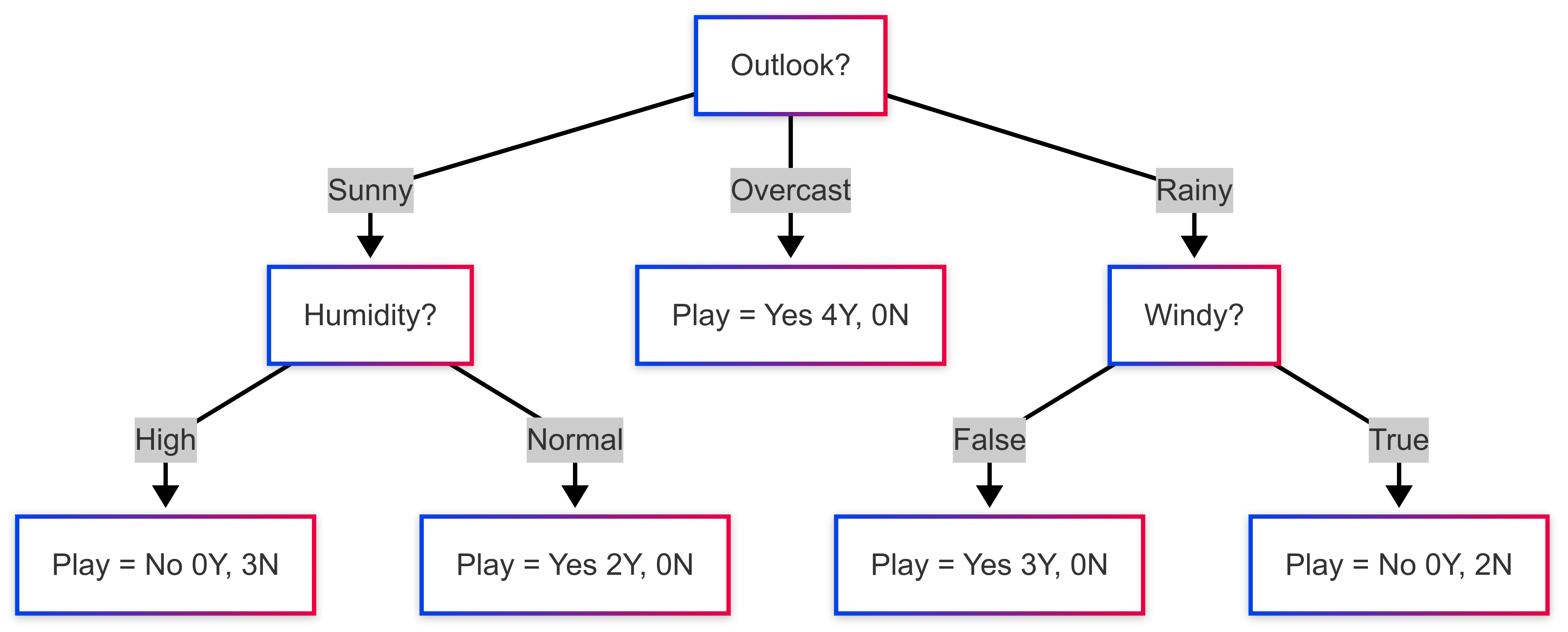
This example demonstrates how the ID3 algorithm uses Information Gain to greedily select attributes and build a decision tree until all leaf nodes are pure (or other stopping criteria are met). If we were using C4.5, we would use Gain Ratio. If using CART, we'd use Gini Gain and all splits would be binary (even for categorical features like Outlook, CART would find the best binary partition e.g., Outlook vs Outlook ).
4.5. Key Differences & When to Use Each
| Feature | ID3 | C4.5 | CART |
|---|---|---|---|
| Splitting | Information Gain (Entropy) | Gain Ratio (Entropy) | Gini Index (Classification), Variance Reduction (Regression) |
| Attribute Types | Categorical | Categorical, Continuous | Categorical, Continuous |
| Splits | Multi-way | Multi-way (categorical), Binary (continuous) | Strictly Binary |
| Missing Values | Basic (ignore/impute) | Sophisticated (fractional instances) | Sophisticated (surrogate splits) |
| Pruning | None | Error-based post-pruning | Cost-complexity post-pruning |
| Output | Decision Tree | Decision Tree or Rule Set | Binary Decision Tree (Class. or Reg.) |
| Bias | Towards multi-valued attributes | Reduced bias (due to Gain Ratio) | Less biased than IG |
When to Use Which (Conceptual Guidance):
- ID3: Rarely used in modern practice due to its limitations (overfitting, only categorical data). Mostly of historical and educational importance.
- C4.5: A robust algorithm that performs well on a variety of datasets. Good choice if you need to handle continuous data and want a method that's less biased by attributes with many values. Its ability to output rules can also be beneficial for interpretability.
- CART: Very popular and forms the basis for many modern ensemble methods like Random Forests and Gradient Boosting. Its binary tree structure is computationally efficient and its pruning mechanism is effective. It's also the natural choice if you are building regression trees.
In practice, most modern libraries (like scikit-learn) implement a version similar to CART (often allowing both "Gini" and "Entropy" criteria for classification), offering a flexible and optimized decision tree builder.
4.6. Pseudocode & Complexity Analysis
General Decision Tree Building Algorithm (Recursive)
Function BuildTree(, ):
-
If all samples in S belong to the same class , or other stopping criteria met (e.g., S is small, F is empty):
- Create a leaf node N.
- Label N with class (e.g., majority class in S).
- Return N.
-
Select the "best" attribute from and its "best" split point/value(s) using a splitting criterion (e.g., maximizing Information Gain, Gain Ratio, or Gini Gain).
-
Create an internal node N.
-
Label N with and .
-
For each outcome of the split (or based on ):
- Let be the subset of where determines outcome .
- If is empty:
- Create a leaf
child_N. - Label
child_Nwith the majority class of . - Add
child_Nas a child ofN.
- Create a leaf
- Else:
- child*N = BuildTree(, ) // Recursively build subtree
- Add child_N as a child of N.
-
Return N.
Stopping Criteria (Examples):
- All samples in the current node belong to the same class.
- No more attributes to split on.
- The number of samples in the node is less than
min_samples_split. - The depth of the tree would exceed
max_depth. - The impurity reduction (gain) is less than
min_impurity_decrease.
Complexity Analysis
Let:
- = number of training examples
- = number of attributes (features)
- = depth of the tree
Tree Construction Phase:
- At each node, to find the best split, we typically iterate through all attributes.
- For each categorical attribute with values, calculating impurity might take (if not already sorted or using histograms).
- For each numerical attribute, data is typically sorted first, which takes . Then, evaluating all possible split points can be done in . So, numerical attributes often dominate this step.
- If all attributes are numerical, finding the best split at one node might take if sorting is done at each node, or if data is pre-sorted or sorting isn't the bottleneck.
- The number of nodes can be up to in the worst case (a skewed tree).
- Thus, a rough upper bound for tree construction can be around or in many practical scenarios, especially if not optimized. More optimized versions (like scikit-learn's, which pre-sorts) can achieve closer to for the entire tree if the depth is not too large. Scikit-learn's implementation has a complexity of for construction.
Prediction Phase (Classifying a new instance):
- Traversing the tree from the root to a leaf node takes .
- In the best case (balanced tree), depth is , where is the number of leaf nodes.
- In the worst case (unbalanced tree, like a linked list), depth can be .
- So, prediction is generally very fast, often or where is tree depth.
These complexities highlight why pruning and setting constraints like max_depth are important not only for generalization but also for managing computational resources.
5. Pruning Methods to Avoid Over-Fitting
One of the major challenges with decision trees is their tendency to overfit the training data. An overfit model learns the training data too well, capturing not only the underlying patterns but also the noise and specific idiosyncrasies of that particular dataset. Such a model will perform exceptionally well on the training data but poorly on new, unseen data (i.e., it has poor generalization).
A decision tree that is grown to its maximum depth, where each leaf node is perfectly pure or contains only unique samples, is highly likely to be overfit. It creates very specific rules that might not hold true for the broader population. Pruning is the process of reducing the size of the decision tree by removing sections (subtrees or branches) that are non-critical or detrimental to generalization performance.
5.1. The Bias–Variance Trade-off in Trees
The problem of overfitting is closely related to the bias–variance trade-off, a fundamental concept in machine learning.
- Bias: Bias refers to the error introduced by approximating a real-world problem, which may be complex, by a much simpler model. A high-bias model makes strong assumptions about the data (e.g., a linear model assuming a linear relationship) and may underfit, failing to capture important patterns. Very shallow decision trees can have high bias.
- Variance: Variance refers to the amount by which the model's learned function would change if it were trained on a different training dataset. A high-variance model is very sensitive to the specific training data; it learns the noise. Complex, deep decision trees tend to have high variance.
An unpruned, fully grown decision tree often has low bias (it can fit the training data very closely) but high variance (it's very specific to the training set and won't generalize well). Pruning aims to find a better balance in this trade-off. By simplifying the tree, we might slightly increase its bias (it might not fit the training data perfectly anymore) but significantly reduce its variance, leading to better overall performance on unseen data.
The goal is to find a tree that is complex enough to capture the true underlying patterns but not so complex that it models the noise.
5.2. Pre-pruning (Early Stopping Criteria)
Pre-pruning, also known as early stopping, involves halting the tree construction process early, before it perfectly classifies the training data. This is done by setting certain stopping criteria during the tree-growing phase. If a split results in a new node that doesn't meet these criteria (or improves upon a certain threshold), the splitting process is stopped, and that node becomes a leaf.
Common pre-pruning criteria include:
-
Maximum Depth (
max_depth): Limit the maximum depth the tree can grow. For instance, ifmax_depthis set to 3, the tree will not have any paths from the root to a leaf longer than 3 splits. This prevents the tree from becoming overly complex and capturing very specific, deep patterns. -
Minimum Samples per Leaf (
min_samples_leaf): Specify the minimum number of training samples a leaf node must contain. If a split would result in a leaf node having fewer samples than this threshold, the split is not performed, and the current node becomes a leaf (even if impure). This prevents the creation of leaves that are based on very few, potentially noisy, examples. -
Minimum Samples per Split (
min_samples_split): Specify the minimum number of training samples a node must have to be considered for splitting. If a node has fewer samples than this threshold, it will not be split further and will become a leaf. -
Minimum Impurity Decrease (
min_impurity_decrease): A node will be split if this split induces a decrease of the impurity greater than or equal to this value. The impurity decrease is the (weighted) Gini gain or Information Gain. If no split can achieve at least this much gain, the node becomes a leaf. This ensures that splits are only made if they significantly improve node purity.
Advantages of Pre-pruning:
- It's computationally efficient because it stops the tree from growing too large, saving time in both training and prediction.
Disadvantages of Pre-pruning:
- It can be "greedy." A decision to stop splitting early might be suboptimal because a seemingly poor split now could lead to very good splits later down the tree. It's hard to determine the optimal stopping points without seeing the fully grown tree.
5.3. Post-pruning (Backward Pruning)
Post-pruning involves growing the decision tree to its full complexity (or near full complexity, perhaps with some basic pre-pruning like min_samples_leaf) and then pruning it backward. It examines nodes and subtrees for removal if they do not contribute significantly to the model's generalization ability, typically by evaluating their impact on a validation dataset or using a complexity measure.
Common post-pruning techniques include:
-
Reduced Error Pruning (REP): This is one of the simplest and most intuitive methods. It works by iterating over each non-leaf node in the fully grown tree. For each node, it considers the effect of replacing its subtree with a leaf node (labeled with the majority class of the samples at that node). If the pruned tree performs no worse (or even better) on a separate validation dataset, the subtree is permanently pruned. This process continues until no further pruning improves accuracy on the validation set.
- Limitation: Requires a separate validation set, which might reduce the amount of data available for training, especially for smaller datasets.
-
Cost-Complexity Pruning (CCP) / Weakest Link Pruning: This method, notably used in the CART algorithm, is more sophisticated. It doesn't just decide to prune or not; it generates a sequence of progressively smaller trees. For a given tree , its cost-complexity is defined as: Where:
- is the misclassification rate (or total impurity like Gini/Entropy sum) of the tree on the training data.
- is the number of terminal nodes (leaves) in the tree .
- () is a complexity parameter that penalizes larger trees. It represents the cost of adding another leaf to the tree.
The algorithm finds, for various values of , the subtree of the initial large tree that minimizes .
- When , the optimal tree is itself (no penalty for complexity).
- As increases, the penalty for complexity increases, leading to smaller pruned trees.
The process involves finding the "weakest link" – the internal node which, if pruned, provides the smallest increase in per pruned leaf. This node and its subtree are pruned, effectively increasing . This generates a sequence of optimal subtrees.
The final step is to select the "best" tree from this sequence, typically by evaluating each tree's performance on a separate validation set or using cross-validation to find the that yields the best generalization. Scikit-learn's
DecisionTreeClassifieruses CCP.
-
Error-Based Pruning (EBP): Used in C4.5, this method estimates the expected error rate of a subtree and its corresponding leaf replacement. It uses a statistical approach (based on binomial confidence intervals) to estimate the error rate if the subtree is replaced by a leaf node. If the estimated error of the leaf is lower than the sum of estimated errors of the subtree's branches, the subtree is pruned.
Advantages of Post-pruning:
- It can consider the overall structure of the tree and make more informed decisions than pre-pruning, often leading to better performing trees.
Disadvantages of Post-pruning:
- It's more computationally expensive because it requires growing a full tree first and then performing pruning operations.
5.4. Practical Tips for Effective Pruning
- Use a Validation Set: Whether pre-pruning or post-pruning, making decisions based on performance on unseen validation data is crucial. A common split is 70% training, 15% validation (for tuning and pruning), and 15% testing (for final evaluation).
- Cross-Validation for : For methods like Cost-Complexity Pruning, use k-fold cross-validation on the training data to find the optimal value of the complexity parameter . This is more robust than using a single validation set, especially with limited data. Scikit-learn does this when you tune
ccp_alpha. - Start with Sensible Pre-pruning Parameters: Even if primarily relying on post-pruning, using some mild pre-pruning (like
min_samples_leaf=5ormax_depth=10-15for moderately sized datasets) can speed up the initial tree growth without sacrificing too much potential quality. - Visualize Tree Depth and Performance: Plot the tree's performance (e.g., accuracy on validation set) against
max_depthorccp_alphato understand how complexity affects generalization. This can help in choosing appropriate parameters. - Consider the Problem: For some problems, interpretability is key, and a smaller, slightly less accurate tree might be preferable to a large, complex one. Pruning helps achieve this.
- Beware of Small Datasets: Pruning decisions are less reliable with very small datasets, as performance on a small validation set can be noisy. More aggressive pre-pruning might be safer, or using ensemble methods could be a better approach altogether.
Pruning is essential for building decision trees that generalize well to new data, transforming a potentially high-variance model into one with a better bias-variance balance.
6. Regression Trees
While our discussion so far has centered on classification trees (predicting categorical outcomes), decision trees are also highly effective for regression tasks, where the goal is to predict a continuous target variable. Examples include predicting house prices, stock values, or a patient's length of stay in a hospital. The CART (Classification and Regression Trees) algorithm, for instance, explicitly supports both types.
The overall structure and building process of a regression tree are very similar to a classification tree:
- It's a binary tree.
- It partitions the feature space recursively.
- Splits are chosen to create more "homogeneous" child nodes.
The key differences lie in:
- How impurity (or error) is measured at a node.
- How predictions are made at the leaf nodes.
6.1. Loss Functions (Measures of Impurity/Error for Regression)
In classification, we used metrics like Gini impurity or entropy to measure node homogeneity. For regression trees, the goal is to minimize the variability of the target variable within the nodes. Common loss functions (or impurity/error measures) used for splitting include:
-
Mean Squared Error (MSE): This is the most widely used criterion. For a node containing a set of samples, the MSE is the average squared difference between the actual values and the mean target value within that node. Let be the target value for instance in node , and be the mean of the target values in node : The MSE for node is: When considering a split, the algorithm chooses the feature and split point that minimize the weighted average MSE of the child nodes. The reduction in MSE is analogous to Gini gain or Information Gain.
-
Mean Absolute Error (MAE) / Least Absolute Deviation (LAD): MAE measures the average absolute difference between the actual values and a central point (typically the median) within the node. Let be the median of the target values in node . (Sometimes the mean is used instead of the median for MAE calculation in some contexts, though median is more robust to outliers for MAE as a loss). MAE is less sensitive to outliers than MSE because it doesn't square the errors. However, MSE is more common due to its mathematical properties (e.g., differentiability).
-
Variance Reduction: Minimizing MSE is equivalent to maximizing variance reduction. The variance of the target variable in a node is: This is identical to MSE. So, splitting criteria are often described as "variance reduction." The split that leads to the largest reduction in variance (parent variance - weighted child variances) is chosen.
6.2. Tree-building with Continuous Targets
The tree-building process for regression trees follows the same top-down, greedy approach:
- Start with all data at the root node. Calculate the "impurity" (e.g., MSE) of the target variable in this node.
- For each attribute:
- If the attribute is categorical: Evaluate all possible binary partitions of its values (similar to CART for classification).
- If the attribute is numerical: Sort the unique values of the attribute. Consider split points (thresholds) typically at the midpoints between successive sorted values.
- For each potential split point:
- Divide the data into two child nodes.
- Calculate the weighted average MSE (or MAE) of the child nodes.
- The split that yields the largest reduction in MSE (or MAE) is chosen as the best split for that attribute.
- Select the attribute and its best split point that result in the overall maximum reduction in MSE (or MAE). This attribute and split point define the split for the current node.
- Recursively repeat steps 2-4 for each child node until a stopping criterion is met (e.g.,
max_depth,min_samples_leaf,min_impurity_decreasewhere impurity is now MSE/MAE).
Prediction at Leaf Nodes: Once the tree is built, a prediction for a new instance is made by traversing the tree down to a leaf node based on the instance's feature values.
- For a regression tree using MSE as the splitting criterion, the prediction at a leaf node is typically the mean of the target variable values of the training instances that fall into that leaf.
- For a regression tree using MAE, the prediction at a leaf node is typically the median of the target variable values in that leaf.
Effectively, a regression tree partitions the feature space into rectangular regions, and assigns a constant predicted value (mean or median) to all instances falling within each region. This results in a step-wise prediction function.
6.3. Pruning & Complexity in Regression Trees
Overfitting is also a significant concern for regression trees. A tree grown too deep will learn the noise in the training data, leading to poor predictions on new data. The pruning techniques discussed for classification trees are directly applicable to regression trees:
-
Pre-pruning (Early Stopping):
max_depth: Limits the tree depth.min_samples_leaf: Ensures each leaf has a minimum number of samples, preventing predictions based on very small, potentially unrepresentative groups.min_samples_split: Requires a node to have a minimum number of samples to be considered for splitting.min_impurity_decrease: Requires a split to reduce the MSE (or MAE) by at least a certain amount. In scikit-learn, this ismin_impurity_decreaseand the impurity used is typically variance (MSE).
-
Post-pruning (e.g., Cost-Complexity Pruning): The Cost-Complexity Pruning (CCP) method used in CART works similarly for regression trees. The cost-complexity function becomes: Where:
- is the sum of squared errors (or total MSE) for all terminal nodes of the tree on the training data.
- is the number of terminal nodes.
- is the complexity parameter. Cross-validation is used to find the optimal that balances the tree's fit to the training data (low MSE) against its complexity (number of leaves).
Complexity Analysis: The computational complexity for building and predicting with regression trees is very similar to that of classification trees.
- Construction: Dominated by sorting numerical features and evaluating splits. Roughly with optimizations for samples and features.
- Prediction: Fast, .
Regression trees provide an interpretable way to model non-linear relationships for continuous target variables and serve as building blocks for more powerful ensemble methods like Random Forest Regressors and Gradient Boosting Regressors.
7. Practical Implementation
Understanding the theory behind decision trees is crucial, but applying them effectively in practice involves several steps, from preparing the data to choosing the right tools and tuning parameters.
7.1. Data Preparation & Feature Encoding
While decision trees are relatively robust to data scaling issues, proper data preparation is still important for optimal performance and to enable the algorithm to work correctly.
-
Handling Missing Values:
- As discussed, some algorithms (like C4.5 and CART) have built-in mechanisms for handling missing values (e.g., fractional instances, surrogate splits).
- If your chosen implementation doesn't handle them natively, or if you prefer a different strategy, you'll need to impute missing values before training. Common strategies include:
- Mean/Median Imputation: Replace missing numerical values with the mean or median of the column.
- Mode Imputation: Replace missing categorical values with the mode (most frequent value) of the column.
- Model-based Imputation: Use another machine learning model (like k-NN or a regression model) to predict and fill in missing values.
- Indicator Variable: Add a binary column indicating whether the original value was missing, and then impute using another method. This allows the tree to potentially learn from the "missingness" itself.
- Alternatively, rows with missing values can be dropped, but this is generally not recommended if it leads to significant data loss.
-
Feature Encoding (for Categorical Features):
- Most decision tree implementations in popular libraries like scikit-learn require numerical input. Therefore, categorical features need to be converted into a numerical format.
- One-Hot Encoding: This is a common method. For a categorical feature with unique values, it creates new binary (0/1) features. Each new feature corresponds to one of the original values. For example, 'Color' with values Blue would become three features:
Is_Red,Is_Green,Is_Blue.- Caution: Can lead to a high number of features if a categorical variable has many unique values (high cardinality), potentially making trees more complex or splits less meaningful.
- Label Encoding: Assigns a unique integer to each category (e.g., Red=0, Green=1, Blue=2).
- Caution: This can inadvertently introduce an ordinal relationship where none exists (e.g., the algorithm might interpret Blue > Green > Red). While tree-based methods can sometimes handle this by finding appropriate split points, it's generally less safe than one-hot encoding for nominal categorical data. It might be acceptable for ordinal categorical features if the encoding reflects the order.
- Other methods: Ordinal encoding (if categories have a natural order), target encoding (encodes categories based on the mean of the target variable for that category – use with care to avoid data leakage).
-
Feature Scaling (Generally Not Required, but can be beneficial for some implementations/visualizations):
- Decision trees make splits based on thresholds for individual features, so the scale of the features (e.g., one feature ranging from 0-1 and another from 0-1000) doesn't directly impact the split logic itself. Unlike distance-based algorithms (like k-NN or SVMs) or gradient descent-based methods, feature scaling (like standardization or normalization) is generally not a strict requirement for decision trees to function correctly.
- However, some implementations or associated processes (like some forms of feature importance visualization or if the tree is part of a pipeline with other algorithms that do require scaling) might implicitly benefit from it. It doesn't usually hurt, but often isn't necessary.
-
Handling Outliers:
- Decision trees are relatively robust to outliers in feature values because splits are based on ordering and thresholding, not on distances that can be heavily skewed by extreme values. An outlier might influence the exact position of a split point, but it's less likely to drastically change the tree structure compared to its effect on, say, linear regression.
- Outliers in the target variable for regression trees can have a more significant impact, especially if using MSE as the splitting criterion.
7.2. Building from Scratch in Python (Conceptual Overview)
While you'll mostly use established libraries, understanding how to build a tree from scratch reinforces the concepts.
import numpy as np

class Node:
    def __init__(self, feature=None, threshold=None, value=None,
                 left_child=None, right_child=None,
                 impurity=None, num_samples=None):
        self.feature = feature
        self.threshold = threshold
        self.value = value
        self.left_child = left_child
        self.right_child = right_child
        self.impurity = impurity
        self.num_samples = num_samples

class DecisionTree:
    def __init__(self, max_depth=None, min_samples_split=2,
                 min_samples_leaf=1, criterion='gini'):
        self.root = None
        self.max_depth = max_depth
        self.min_samples_split = min_samples_split
        self.min_samples_leaf = min_samples_leaf
        self.criterion = criterion

    def _calculate_impurity(self, y):
        """Gini, Entropy (classification) or MSE (regression)."""
        m = y.shape[0]
        if m == 0:
            return 0
        if self.criterion == 'gini':
            counts = np.bincount(y)
            ps = counts / m
            impurity = 1.0 - np.sum(ps**2)
        elif self.criterion == 'entropy':
            counts = np.bincount(y)
            ps = counts / m
            ps = ps[ps > 0]
            impurity = -np.sum(ps * np.log2(ps))
        elif self.criterion == 'mse':
            mean_y = np.mean(y)
            impurity = np.mean((y - mean_y)**2)
        else:
            raise ValueError(f"Unknown criterion {self.criterion}")
        return impurity

    def _find_best_split(self, X, y):
        """Find the best feature and threshold to split on."""
        m, n_features = X.shape
        if m < 2:
            return None, None

        parent_impurity = self._calculate_impurity(y)
        best_gain = -1.0
        best_feat, best_thr = None, None

        for feat_idx in range(n_features):
            X_col = X[:, feat_idx]
            unique_vals = np.unique(X_col)
            if unique_vals.shape[0] <= 1:
                continue
            # candidate thresholds: midpoints
            thresholds = (unique_vals[:-1] + unique_vals[1:]) / 2.0
            for thr in thresholds:
                left_mask = X_col < thr
                right_mask = ~left_mask
                n_left = np.sum(left_mask)
                n_right = np.sum(right_mask)
                if n_left < self.min_samples_leaf or n_right < self.min_samples_leaf:
                    continue
                y_left, y_right = y[left_mask], y[right_mask]
                imp_left = self._calculate_impurity(y_left)
                imp_right = self._calculate_impurity(y_right)
                # weighted impurity
                child_imp = (n_left * imp_left + n_right * imp_right) / m
                gain = parent_impurity - child_imp
                if gain > best_gain:
                    best_gain = gain
                    best_feat = feat_idx
                    best_thr = thr

        return best_feat, best_thr

    def _calculate_leaf_value(self, y):
        """Return majority class (classification) or mean (regression)."""
        if self.criterion in ('gini', 'entropy'):
            counts = np.bincount(y)
            return np.argmax(counts)
        else:  # mse
            return np.mean(y)

    def _build_tree_recursive(self, X, y, depth):
        num_samples, _ = X.shape
        # stopping conditions
        if (depth >= self.max_depth if self.max_depth is not None else False or
            num_samples < self.min_samples_split or
            (self.criterion in ('gini', 'entropy') and len(np.unique(y)) == 1)):
            leaf_val = self._calculate_leaf_value(y)
            return Node(value=leaf_val,
                        impurity=self._calculate_impurity(y),
                        num_samples=num_samples)

        feat, thr = self._find_best_split(X, y)
        if feat is None:
            leaf_val = self._calculate_leaf_value(y)
            return Node(value=leaf_val,
                        impurity=self._calculate_impurity(y),
                        num_samples=num_samples)

        # split data
        left_mask = X[:, feat] < thr
        right_mask = ~left_mask
        if (np.sum(left_mask) < self.min_samples_leaf or
            np.sum(right_mask) < self.min_samples_leaf):
            leaf_val = self._calculate_leaf_value(y)
            return Node(value=leaf_val,
                        impurity=self._calculate_impurity(y),
                        num_samples=num_samples)

        X_left, y_left = X[left_mask], y[left_mask]
        X_right, y_right = X[right_mask], y[right_mask]

        left_sub = self._build_tree_recursive(X_left, y_left, depth + 1)
        right_sub = self._build_tree_recursive(X_right, y_right, depth + 1)

        return Node(feature=feat, threshold=thr,
                    left_child=left_sub, right_child=right_sub,
                    impurity=self._calculate_impurity(y),
                    num_samples=num_samples)

    def fit(self, X, y):
        """Build decision tree classifier/regressor."""
        X = np.array(X)
        y = np.array(y)
        self.root = self._build_tree_recursive(X, y, depth=0)

    def _predict_instance(self, x, node):
        if node.value is not None:
            return node.value
        if x[node.feature] < node.threshold:
            return self._predict_instance(x, node.left_child)
        else:
            return self._predict_instance(x, node.right_child)

    def predict(self, X):
        X = np.array(X)
return np.array([self._predict_instance(x, self.root) for x in X])To experiment with this implementation, you can access and test the code at this Kaggle notebook: https://www.kaggle.com/code/ayushrudani/decision-tree-classification-implementation
This conceptual code outlines the main components but omits many details (like efficient splitting for numerical features, handling various categorical split types, and robust impurity calculations). Building a production-ready tree from scratch is a substantial undertaking.
7.3. Using scikit-learn’s DecisionTreeClassifier / DecisionTreeRegressor
For most practical purposes, you'll use well-optimized libraries like scikit-learn.
Classification Example:
from sklearn.tree import DecisionTreeClassifier
from sklearn.model_selection import train_test_split
from sklearn.metrics import accuracy_score
from sklearn.datasets import load_iris
from sklearn.preprocessing import LabelEncoder # If target is string
import pandas as pd

# Load a sample dataset (e.g., Iris)
iris = load_iris()
X, y = iris.data, iris.target
# Feature names: iris.feature_names
# Class names: iris.target_names

# Split data
X_train, X_test, y_train, y_test = train_test_split(X, y, test_size=0.3, random_state=42)

# Initialize the classifier
# Common hyperparameters:
# - criterion: "gini" (default) or "entropy"
# - max_depth: Maximum depth of the tree (pre-pruning)
# - min_samples_split: Minimum samples required to split an internal node (pre-pruning)
# - min_samples_leaf: Minimum samples required to be at a leaf node (pre-pruning)
# - ccp_alpha: Complexity parameter for Minimal Cost-Complexity Pruning (post-pruning)
clf = DecisionTreeClassifier(criterion='gini', max_depth=3, random_state=42)

# Train the model
clf.fit(X_train, y_train)

# Make predictions
y_pred = clf.predict(X_test)

# Evaluate the model
accuracy = accuracy_score(y_test, y_pred)
print(f"Accuracy: {accuracy:.4f}")

# To visualize the tree (requires graphviz and matplotlib)
from sklearn.tree import plot_tree
import matplotlib.pyplot as plt

plt.figure(figsize=(20,10))
plot_tree(clf, filled=True, feature_names=iris.feature_names, class_names=list(iris.target_names.astype(str)), rounded=True)
plt.show()
Regression Example:
from sklearn.tree import DecisionTreeRegressor
from sklearn.model_selection import train_test_split
from sklearn.metrics import mean_squared_error
import numpy as np
import matplotlib.pyplot as plt

# Create a sample regression dataset
rng = np.random.RandomState(1)
X = np.sort(5 * rng.rand(80, 1), axis=0)
y = np.sin(X).ravel()
y[::5] += 3 * (0.5 - rng.rand(16)) # Add some noise

X_train, X_test, y_train, y_test = train_test_split(X, y, test_size=0.3, random_state=42)

# Initialize the regressor
# criterion: "squared_error" (default, formerly "mse"), "friedman_mse", "absolute_error" a(MAE), "poisson"
reg = DecisionTreeRegressor(max_depth=3, random_state=42, criterion="squared_error")

# Train the model
reg.fit(X_train, y_train)

# Make predictions
y_pred = reg.predict(X_test)

# Evaluate the model
mse = mean_squared_error(y_test, y_pred)
print(f"Mean Squared Error: {mse:.4f}")

# Visualize (for 1D feature regression)
plt.figure(figsize=(10,6))
plt.scatter(X, y, s=20, edgecolor="black", c="darkorange", label="data")
X_plot = np.arange(0.0, 5.0, 0.01)[:, np.newaxis]
y_plot = reg.predict(X_plot)
plt.plot(X_plot, y_plot, color="cornflowerblue", label="prediction", linewidth=2)
plt.xlabel("data")
plt.ylabel("target")
plt.title("Decision Tree Regression")
plt.legend()
plt.show()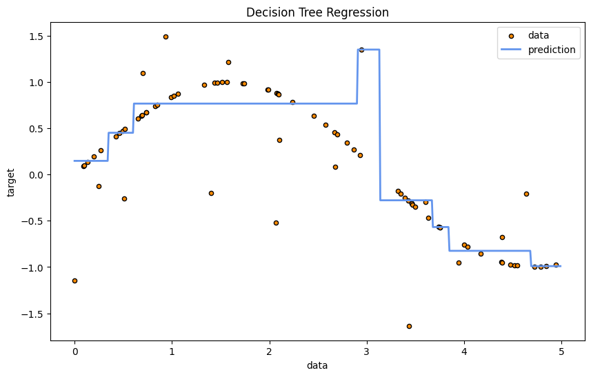
7.4. Hyperparameter Tuning (GridSearchCV)
Finding the optimal hyperparameters (like max_depth, min_samples_leaf, ccp_alpha) is crucial for building a good decision tree model that generalizes well. Scikit-learn's GridSearchCV can automate this process.
from sklearn.tree import DecisionTreeClassifier, DecisionTreeRegressor
from sklearn.model_selection import GridSearchCV
from sklearn.metrics import accuracy_score, mean_squared_error

# Define the parameter grid for DecisionTreeClassifier
param_grid_clf = {
    'criterion': ['gini', 'entropy'],
    'max_depth': [None, 3, 5, 7, 10],
    'min_samples_split': [2, 5, 10],
    'min_samples_leaf': [1, 2, 4],
    'ccp_alpha': [0.0, 0.001, 0.005, 0.01, 0.02]
}

grid_search_clf = GridSearchCV(
    DecisionTreeClassifier(random_state=42),
    param_grid_clf,
    cv=5,
    scoring='accuracy',
    verbose=1,
    n_jobs=-1
)
grid_search_clf.fit(X_train, y_train)

print("Best parameters for Classifier:", grid_search_clf.best_params_)
best_clf = grid_search_clf.best_estimator_
y_pred_best_clf = best_clf.predict(X_test)
print(f"Best Classifier Accuracy: "
      f"{accuracy_score(y_test, y_pred_best_clf):.4f}")

# Define the parameter grid for DecisionTreeRegressor
param_grid_reg = {
    'criterion': ['squared_error', 'absolute_error'],
    'max_depth': [None, 3, 5, 7, 10],
    'min_samples_split': [2, 5, 10, 20],
    'min_samples_leaf': [1, 2, 5, 10]
}

grid_search_reg = GridSearchCV(
    DecisionTreeRegressor(random_state=42),
    param_grid_reg,
    cv=5,
    scoring='neg_mean_squared_error',
    verbose=1,
    n_jobs=-1
)
grid_search_reg.fit(X_train, y_train)

print("Best parameters for Regressor:", grid_search_reg.best_params_)
best_reg = grid_search_reg.best_estimator_
y_pred_best_reg = best_reg.predict(X_test)
print(f"Best Regressor MSE: "
      f"{mean_squared_error(y_test, y_pred_best_reg):.4f}")
When tuning ccp_alpha, it's often beneficial to first compute the effective alphas using cost_complexity_pruning_path and use those values in your grid search, rather than arbitrary small numbers. This makes the search more targeted.
This section provides a practical guide to implementing decision trees, highlighting key steps and tools.
8. Model Evaluation
Once a decision tree model is trained, evaluating its performance is crucial to understand its effectiveness and to compare it with other models or different hyperparameter settings. Evaluation is typically performed on a hold-out test set (data not seen during training or hyperparameter tuning).
8.1. Confusion Matrix & Derived Metrics (for Classification)
For classification tasks, the Confusion Matrix is a cornerstone of model evaluation. It provides a detailed breakdown of correct and incorrect predictions for each class. For a binary classification problem (e.g., Positive/Negative), it looks like this:
| Predicted Positive | Predicted Negative | |
|---|---|---|
| Actual Positive | True Positive (TP) | False Negative (FN) |
| Actual Negative | False Positive (FP) | True Negative (TN) |
- True Positive (TP): Instances correctly predicted as Positive.
- False Negative (FN): Instances incorrectly predicted as Negative (Type II error).
- False Positive (FP): Instances incorrectly predicted as Positive (Type I error).
- True Negative (TN): Instances correctly predicted as Negative.
From the confusion matrix, several key performance metrics can be derived:
-
Accuracy: The proportion of total predictions that were correct. While common, accuracy can be misleading, especially with imbalanced datasets (where one class is much more frequent than others).
-
Precision (Positive Predictive Value - PPV): Of all instances predicted as Positive, what proportion was actually Positive? Measures the exactness of the positive predictions. High precision means fewer false positives. Useful when the cost of a False Positive is high (e.g., spam detection – you don't want to mark a legitimate email as spam).
-
Recall (Sensitivity, True Positive Rate - TPR): Of all actual Positive instances, what proportion was correctly predicted as Positive? Measures the completeness of positive predictions. High recall means fewer false negatives. Useful when the cost of a False Negative is high (e.g., medical diagnosis – you don't want to miss a disease).
-
Specificity (True Negative Rate - TNR): Of all actual Negative instances, what proportion was correctly predicted as Negative?
-
F1-Score: The harmonic mean of Precision and Recall. It provides a single score that balances both concerns. It's particularly useful when you need a balance between Precision and Recall, especially if there's an uneven class distribution.
-
Matthews Correlation Coefficient (MCC): A robust measure that takes into account all four values in the confusion matrix. It's considered a balanced measure even for imbalanced classes. Values range from -1 (total disagreement) to +1 (perfect agreement), with 0 being random prediction.
When dealing with multi-class classification, these metrics can be extended (e.g., macro-average, micro-average, weighted-average precision/recall/F1).
8.2. ROC Curve & AUC
The Receiver Operating Characteristic (ROC) curve and the Area Under the Curve (AUC) are powerful tools for evaluating binary classifiers, especially when class balance is a concern or when you want to understand performance across different decision thresholds.
-
ROC Curve: The ROC curve plots the True Positive Rate (TPR) (Recall/Sensitivity) against the False Positive Rate (FPR) at various threshold settings. FPR is calculated as: Most decision tree classifiers output probabilities (or scores that can be converted to probabilities) for class membership. By varying the threshold for classifying an instance as "Positive" (e.g., if probability > threshold, predict Positive), we get different pairs of (TPR, FPR), which trace out the ROC curve.
- A perfect classifier would have a point at (0,1) (FPR=0, TPR=1).
- A random classifier (like flipping a coin) would produce a diagonal line from (0,0) to (1,1).
- The closer the ROC curve is to the top-left corner, the better the classifier's performance.
-
Area Under the Curve (AUC): The AUC quantifies the overall ability of the classifier to distinguish between positive and negative classes. It represents the probability that the classifier will rank a randomly chosen positive instance higher than a randomly chosen negative instance.
- AUC = 1: Perfect classifier.
- AUC = 0.5: Random classifier (no discriminative power).
- AUC < 0.5: Classifier is performing worse than random (check for flipped labels or model issues). AUC is useful because it provides a single scalar value summarizing performance across all thresholds and is insensitive to class imbalance.
8.3. Cross-Validation & Learning Curves
-
Cross-Validation (CV): Relying on a single train-test split can lead to a noisy estimate of model performance, especially with smaller datasets. k-fold Cross-Validation is a more robust technique:
- The training data is divided into equal (or nearly equal) folds.
- The model is trained times. In each iteration, folds are used for training, and the remaining fold is used for validation (testing).
- The performance metric (e.g., accuracy, F1-score, AUC) is calculated for each fold.
- The average of these metrics (and its standard deviation) provides a more stable and reliable estimate of the model's generalization performance.
Common values for are 5 or 10. Cross-validation is also crucial during hyperparameter tuning (as seen with
GridSearchCV) to ensure that the chosen hyperparameters generalize well.
-
Learning Curves: Learning curves help diagnose issues like bias and variance in the model. They plot a performance metric (e.g., accuracy or error) against the amount of training data used. Typically, two curves are plotted:
- Training Score: Performance on the training data used.
- Validation Score (Cross-Validation Score): Performance on a held-out validation set (or average from cross-validation).
Interpreting Learning Curves:
- High Bias (Underfitting): If both training and validation scores are low and converge to a similar low value as training data size increases, the model is likely too simple and underfitting. More data won't significantly help; a more complex model or better features are needed.
- High Variance (Overfitting): If there's a large gap between a high training score and a lower validation score, the model is likely overfitting. The training score might keep increasing, while the validation score plateaus or even decreases. More data can help reduce overfitting. Pruning, reducing model complexity, or regularization are also solutions.
- Ideal: Both scores converge to a high value, and the gap between them is small.
By employing these evaluation techniques, you can gain a comprehensive understanding of your decision tree's strengths and weaknesses, ensuring it's well-suited for the task at hand. For regression trees, evaluation would focus on metrics like Mean Squared Error (MSE), Root Mean Squared Error (RMSE), Mean Absolute Error (MAE), and (R-squared or coefficient of determination), often also using cross-validation and learning curves (plotting error metrics).
9. Extensions & Variants
While standard decision trees (like ID3, C4.5, CART) are foundational, their predictive power can sometimes be improved, and their tendency to overfit can be mitigated by using them as building blocks in more complex ensemble methods or by modifying their basic structure.
9.1. Random Forests
A Random Forest is an ensemble learning method that constructs a multitude of decision trees at training time and outputs the class that is the mode of the classes (for classification) or mean/average prediction (for regression) of the individual trees. It's a form of "bagging" (Bootstrap Aggregating) with an added layer of randomness in feature selection.
How it Works:
-
Bootstrap Sampling (Bagging):
- From the original training dataset of samples, multiple (e.g., samples, where is the number of trees) bootstrap samples are created. Each bootstrap sample is created by randomly sampling instances from the original dataset with replacement. This means some instances may appear multiple times in a sample, while others may not appear at all.
- Each bootstrap sample is roughly the same size as the original dataset. On average, about 63.2% of the original instances are included in each bootstrap sample (the remaining ~36.8% are "out-of-bag" instances).
-
Random Feature Selection for Splits:
- A decision tree is grown for each bootstrap sample.
- However, when determining the best split at each node of a tree, instead of considering all available features, Random Forest considers only a random subset of features (where , total number of features). A common choice for is for classification and for regression.
- The best split is then chosen from this random subset of features.
-
Tree Growth:
- The individual trees are typically grown to their maximum depth without pruning (or with minimal pruning like
min_samples_leaf). The ensemble nature and randomness help to control overfitting.
- The individual trees are typically grown to their maximum depth without pruning (or with minimal pruning like
-
Prediction (Aggregation):
- Classification: For a new instance, each tree in the forest predicts a class. The final prediction is the majority vote among all trees.
- Regression: For a new instance, each tree predicts a continuous value. The final prediction is the average of the predictions from all trees.
Advantages of Random Forests:
- High Accuracy: Generally, they provide higher accuracy than individual decision trees and are robust to overfitting.
- Handles High Dimensionality Well: Effective even when the number of features is much larger than the number of samples.
- Feature Importance: Can provide a robust estimate of feature importance by averaging the impurity decrease across all trees or by using permutation importance on out-of-bag samples.
- Handles Missing Data: Can impute missing values during training (though pre-imputation is common).
- Implicit Out-of-Bag (OOB) Error Estimation: The instances not included in a particular bootstrap sample (OOB instances) can be used as a built-in validation set to estimate the model's generalization error without needing a separate validation set.
Disadvantages:
- Less Interpretable: A forest of many trees is much harder to visualize and interpret than a single decision tree ("black box" tendency, though feature importance helps).
- Computationally More Expensive: Training many trees can be time-consuming and memory-intensive compared to a single tree.
9.2. Gradient-Boosted Trees (GBT)
Gradient Boosting is another powerful ensemble technique that builds trees sequentially, where each new tree attempts to correct the errors made by the previously built trees. Unlike Random Forests where trees are built independently, GBTs are built in an additive, stage-wise fashion.
How it Works (Conceptual Overview for a Generic Loss Function):
- Initialize Model: Start with a simple initial model, often a constant value (e.g., the mean of the target variable for regression, or log-odds for classification).
- Iterative Tree Building: For (number of trees): a. Compute Pseudo-Residuals: Calculate the "errors" or "residuals" of the current ensemble's predictions with respect to the true target values. For squared error loss in regression, these are simply (actual - predicted). For other loss functions (like logistic loss for classification), these are gradients of the loss function. b. Fit a New Tree: Train a new (typically small, shallow) decision tree to predict these pseudo-residuals (not the original target variable). This tree learns the patterns in the errors. c. Update Ensemble: Add the predictions of this new tree to the current ensemble's predictions, often scaled by a learning rate (or shrinkage parameter, , typically small, e.g., 0.01-0.1). The learning rate controls the contribution of each tree and helps prevent overfitting.
- Final Prediction: The final prediction is the sum of the initial model's prediction and the contributions from all subsequently added trees (scaled by the learning rate).
Key GBT Variants:
- AdaBoost (Adaptive Boosting): An earlier boosting algorithm often used with shallow decision trees (stumps). It re-weights instances at each iteration, giving higher weight to incorrectly classified instances.
- Gradient Boosting Machine (GBM): The general framework described above.
- XGBoost (Extreme Gradient Boosting): A highly optimized and popular implementation of gradient boosting, known for its speed, performance, and features like regularization, handling missing values, and parallel processing.
- LightGBM (Light Gradient Boosting Machine): Another fast, distributed, high-performance GBT framework, particularly efficient with large datasets. It uses gradient-based one-side sampling (GOSS) and exclusive feature bundling (EFB).
- CatBoost: A GBT library that excels at handling categorical features automatically and effectively, often outperforming others when many categorical features are present.
Advantages of Gradient-Boosted Trees:
- State-of-the-Art Performance: Often achieves top performance on many structured/tabular data problems.
- Flexibility: Can optimize for various loss functions.
- Handles Different Data Types: Can work with numerical and categorical features (though some implementations require pre-processing).
Disadvantages:
- Sensitive to Hyperparameters: Requires careful tuning of parameters like the number of trees, learning rate, tree depth, etc. Can overfit if not tuned properly.
- Slower Training (than Random Forests): Trees are built sequentially, which can be slower than the parallel tree building in Random Forests (though highly optimized libraries like XGBoost and LightGBM mitigate this significantly).
- Less Interpretable (than single trees): Like Random Forests, but feature importance can still be extracted.
9.3. Oblique & Hybrid Trees
Standard decision trees (like those in ID3, C4.5, CART) are "axis-parallel" because their splits are based on a single feature at a time (e.g., Age < 30 or Color = 'Red'). These splits create decision boundaries that are parallel to the feature axes.
-
Oblique Decision Trees: Oblique decision trees allow splits based on a linear combination of multiple features at each internal node. For example, a split could be of the form .
- Decision Boundaries: This allows for "oblique" or "angled" decision boundaries, which can capture correlations and linear relationships between features more efficiently, potentially leading to smaller and more accurate trees, especially when the true underlying decision boundary is not axis-parallel.
- Complexity: Finding the optimal oblique split (i.e., the best weights and threshold) is much more computationally challenging than finding an axis-parallel split. Various heuristic methods are used, such as simulated annealing, genetic algorithms, or linear discriminant analysis at each node.
- Usage: Less common in standard practice than axis-parallel trees due to their increased complexity and computational cost, but they can be very powerful for certain types of data.
-
Hybrid Trees (Model Trees): Hybrid trees, also known as model trees, combine decision tree structures with other types of models at the leaf nodes.
- Instead of assigning a constant class label (classification) or a constant value (regression) to a leaf node, a model tree fits a different model (e.g., a linear regression model) to the instances that reach that leaf.
- Regression Example (M5 Algorithm):
- The tree is grown using a splitting criterion that minimizes intra-subset variation (like standard regression trees).
- Once the tree is grown, a multivariate linear regression model is built for the data in each leaf node, using only the features relevant to that subset (or all features).
- Pruning is then performed by replacing subtrees with linear regression models if the model gives a lower estimated error.
- Advantages: Can provide smoother and more accurate predictions for regression tasks, especially when the underlying data has local linear trends. Can also be more compact than a standard regression tree that tries to approximate a linear function with many small steps.
- Usage: More common in regression contexts. Algorithms like M5 and its variants (e.g., M5P, Cubist) implement these ideas.
These extensions and variants highlight the versatility of the decision tree concept, enabling the creation of highly accurate and robust models for a wide range of machine learning tasks.
10. Best Practices & Common Pitfalls
Building effective decision tree models goes beyond just calling a fit method. Adhering to best practices and being aware of common pitfalls can significantly improve your model's performance, interpretability, and reliability.
10.1. Handling Imbalanced Data
Imbalanced datasets, where one class is significantly more frequent than others, pose a common challenge for many machine learning algorithms, including decision trees. Standard decision tree algorithms aim to maximize overall accuracy (or minimize impurity like Gini/Entropy), which can lead them to be biased towards the majority class. A tree might achieve high accuracy by simply predicting the majority class for most instances, while performing poorly on the minority class, which is often the class of interest (e.g., fraud detection, rare disease diagnosis).
Pitfalls:
- Poor Minority Class Performance: The tree might not learn effective rules to identify the minority class, leading to high false negatives.
- Misleading Evaluation Metrics: Accuracy becomes a poor indicator of performance. A model predicting the majority class 95% of the time will have 95% accuracy, even if it completely fails to identify any minority class instances.
Best Practices:
-
Choose Appropriate Evaluation Metrics:
- Focus on metrics like Precision, Recall, F1-Score (especially for the minority class), AUC-ROC, AUC-PR (Area Under Precision-Recall Curve), and Matthews Correlation Coefficient (MCC). These provide a better picture of performance on imbalanced data than raw accuracy.
-
Resampling Techniques:
- Oversampling the Minority Class: Increase the number of instances in the minority class.
- Random Oversampling: Duplicate random instances from the minority class. Can lead to overfitting on the minority class.
- SMOTE (Synthetic Minority Over-sampling Technique): Generate synthetic samples for the minority class by interpolating between existing minority instances and their nearest neighbors. More sophisticated than random oversampling.
- Undersampling the Majority Class: Decrease the number of instances in the majority class.
- Random Undersampling: Remove random instances from the majority class. Can lead to loss of valuable information from the majority class.
- Tomek Links: Remove pairs of instances (one from each class) that are close to each other and are considered Tomek links (potential noise or borderline cases).
- NearMiss: Selects majority class samples whose average distance to some K-nearest minority class samples is small.
- Combination of Oversampling and Undersampling: Techniques like SMOTE-Tomek or SMOTE-ENN combine both approaches.
- Oversampling the Minority Class: Increase the number of instances in the minority class.
-
Cost-Sensitive Learning:
- Assign different misclassification costs to different classes. Many decision tree implementations (like scikit-learn's
DecisionTreeClassifier) allow you to specify class weights using theclass_weightparameter. Settingclass_weight='balanced'automatically adjusts weights inversely proportional to class frequencies. - This makes the algorithm pay more attention to minimizing errors on the minority class by penalizing its misclassification more heavily.
- Assign different misclassification costs to different classes. Many decision tree implementations (like scikit-learn's
-
Algorithm-Level Approaches:
- Some decision tree variants or ensemble methods are inherently better at handling imbalanced data or have specific modifications for it.
- Ensemble methods like Balanced Random Forests or RUSBoost (Random Undersampling Boost) are specifically designed for imbalanced learning.
-
Generate More Data (If Possible):
- While often not feasible, acquiring more data, especially for the minority class, is the most direct way to address imbalance.
-
Anomaly Detection Approach:
- If the minority class is extremely rare and represents anomalous behavior, framing the problem as anomaly detection rather than classification might be more appropriate.
10.2. Dealing with High-Cardinality Features
High-cardinality features are categorical features with a very large number of unique values (e.g., zip codes, user IDs, product codes). These can pose problems for decision trees:
Pitfalls:
- Overfitting: Trees can create very specific splits for each unique value (or small groups of values), leading to branches that only apply to a few training instances and don't generalize well. Information Gain tends to favor such attributes.
- Increased Tree Complexity: Leads to very wide and deep trees, making them hard to interpret and potentially slow to train/predict.
- Sparsity Issues: One-hot encoding high-cardinality features can result in a massive number of sparse features, increasing memory usage and computational load.
- Data Fragmentation: The data gets split into many small subsets quickly, making subsequent splits less reliable.
Best Practices:
-
Feature Engineering Value Grouping:
- Domain Knowledge: Group categories based on domain expertise (e.g., group zip codes by region, product codes by product type).
- Frequency-based Grouping: Group infrequent categories into a single "Other" or "Rare" category. Set a threshold (e.g., categories appearing in
<1%of instances go into "Other"). - Target-based Grouping: Group categories based on their relationship with the target variable (e.g., group categories with similar average target values in regression, or similar class distributions in classification). Be very careful to do this on a separate training fold to avoid data leakage if using the target directly.
-
Encoding Techniques:
- Target Encoding (Mean Encoding): Replace each category with the mean of the target variable for that category.
- Pros: Can be very effective as it directly incorporates information about the target.
- Cons: Prone to overfitting and data leakage if not implemented carefully (e.g., must be done within cross-validation folds, or use smoothing techniques).
- Weight of Evidence (WoE) Encoding: Similar to target encoding, often used in credit scoring. It measures the "strength" of a category in separating good and bad outcomes. Requires careful handling to prevent leakage.
- Hashing Encoding (Feature Hashing): Hashes category names into a fixed number of output features. Can handle arbitrary numbers of categories with controlled output dimensionality.
- Pros: Low memory, fast.
- Cons: Hash collisions (different categories mapping to the same hash) can occur, potentially losing information. Interpretability is reduced.
- Embedding Layers (for very high cardinality, usually with Neural Networks): Learn a dense vector representation (embedding) for each category. Less common for standalone decision trees but useful in more complex pipelines.
- Target Encoding (Mean Encoding): Replace each category with the mean of the target variable for that category.
-
Tree Algorithm Parameters:
- Use algorithms or settings that are less susceptible to high-cardinality bias. C4.5's Gain Ratio helps mitigate this somewhat compared to ID3's Information Gain.
- Utilize pre-pruning parameters like
min_samples_leaformin_samples_spliteffectively. If a split on a high-cardinality feature results in leaves with very few samples, these parameters can prevent such splits.
-
Feature Selection:
- If a high-cardinality feature doesn't add much predictive power after attempting grouping or better encoding, consider removing it.
-
Specialized Tree Variants:
- Some tree variants or libraries (like CatBoost) have built-in sophisticated ways to handle categorical features, including high-cardinality ones, often outperforming standard one-hot encoding.
10.3. Balancing Interpretability vs. Accuracy
One of the primary appeals of decision trees is their interpretability. However, achieving the highest possible accuracy often involves growing complex trees or using ensemble methods like Random Forests or Gradient Boosted Trees, which sacrifice this direct interpretability.
The Trade-off:
- Simple Trees (e.g., shallow depth):
- Pros: Easy to understand, visualize, and explain the decision process.
- Cons: May have lower accuracy (higher bias) as they might not capture complex relationships in the data. Can underfit.
- Complex Trees (e.g., deep, many leaves) / Ensembles:
- Pros: Often achieve higher accuracy and better generalization (lower variance, especially for ensembles).
- Cons: Become "black boxes." Understanding why a specific prediction is made becomes difficult. A single deep tree can be hard to follow; a forest of hundreds of trees is virtually impossible to inspect manually.
Best Practices for Balancing:
-
Define Project Goals:
- Is peak predictive accuracy the absolute priority, or is understanding the decision-making process equally or more important (e.g., in regulated industries, medical diagnosis explanations)? This will guide your choice.
-
Start Simple:
- Begin with a simpler, interpretable tree. Tune its hyperparameters (like
max_depth,min_samples_leaf) to get a baseline understanding and performance. - Visualize this tree and analyze its decision rules.
- Begin with a simpler, interpretable tree. Tune its hyperparameters (like
-
Iteratively Increase Complexity if Needed:
- If the simple tree's performance is insufficient, gradually increase its complexity or consider ensemble methods.
- Monitor the gain in accuracy against the loss in interpretability.
-
Use Post-Hoc Explanation Techniques for Complex Models:
- If high accuracy demands a complex model (like Random Forest or XGBoost), use model-agnostic interpretability techniques:
- Feature Importance: Most tree-based ensembles provide global feature importance scores (e.g., Gini importance, permutation importance), indicating which features contribute most to predictions.
- SHAP (SHapley Additive exPlanations): Provides insights into how each feature contributes to individual predictions (local interpretability) and overall model behavior.
- LIME (Local Interpretable Model-agnostic Explanations): Explains individual predictions by approximating the complex model locally with a simpler, interpretable model (e.g., a linear model or a small tree).
- Partial Dependence Plots (PDP) / Individual Conditional Expectation (ICE) Plots: Show the marginal effect of one or two features on the predicted outcome of a model.
- If high accuracy demands a complex model (like Random Forest or XGBoost), use model-agnostic interpretability techniques:
-
Surrogate Trees:
- Train a simpler, interpretable decision tree to mimic the predictions of a more complex black-box model on a given dataset. The surrogate tree won't be as accurate as the original model but can provide an approximate understanding of its behavior.
-
Pruning:
- Proper pruning (especially cost-complexity pruning) is key to finding a good balance. It simplifies the tree by removing less informative branches, which can improve both generalization and interpretability without a drastic hit on accuracy (sometimes even improving it).
-
Rule Extraction from Trees:
- Even from a moderately complex tree, paths from root to leaf can be translated into IF-THEN rules, which are often easier for humans to digest than the full tree structure.
By consciously considering these aspects, you can navigate the common challenges in decision tree modeling and make informed choices that align with your project's specific requirements for both performance and understanding.
11. Conclusion & Further Reading
We've journeyed through the intricate world of decision trees, exploring their theoretical underpinnings, practical implementation, and the broader ecosystem of techniques that enhance their power. Decision trees, in their various forms, remain a cornerstone of machine learning due to their interpretability, versatility, and effectiveness as standalone models or as components in powerful ensembles.
11.1. Recap of Key Concepts
Let's briefly revisit the core ideas covered:
- Fundamentals: Decision trees are supervised learning models that partition data based on feature values to make predictions. They mimic human-like decision-making processes.
- Purity Measures & Splitting Criteria: We explored how Entropy, Gini Index, and Classification Error quantify node impurity, and how Information Gain, Gain Ratio, and Gini Gain guide the selection of optimal splits.
- Tree-Building Algorithms: Key algorithms like ID3 (Information Gain), C4.5 (Gain Ratio), and CART (Gini Index for classification, MSE for regression) were discussed, each with its specific mechanisms for handling data types and tree construction (e.g., CART's binary splits).
- Overfitting and Pruning: The critical problem of overfitting was addressed, along with techniques like pre-pruning (early stopping criteria like
max_depth,min_samples_leaf) and post-pruning (e.g., Reduced Error Pruning, Cost-Complexity Pruning) to improve generalization. - Regression Trees: We saw how decision trees can be adapted for regression tasks by using error measures like Mean Squared Error (MSE) for splitting and predicting mean values at leaf nodes.
- Practical Implementation: Data preparation (missing values, feature encoding), using libraries like scikit-learn, and hyperparameter tuning (e.g., with GridSearchCV) are essential for effective application.
- Model Evaluation: Metrics such as the confusion matrix, precision, recall, F1-score, ROC-AUC for classification, and MSE/MAE/ for regression, along with cross-validation and learning curves, are vital for assessing model performance.
- Extensions & Variants: The power of decision trees is amplified in ensemble methods like Random Forests (bagging with random feature selection) and Gradient Boosted Trees (sequential error correction), and through structural variants like oblique trees.
- Best Practices: We discussed strategies for handling imbalanced data, managing high-cardinality features, and navigating the trade-off between model interpretability and predictive accuracy.
Decision trees offer a transparent approach to modeling complex data. While a single tree might sometimes be outperformed in raw accuracy by more complex models, its ability to provide clear, understandable rules is invaluable in many contexts. Furthermore, their role as the foundation for highly accurate ensemble methods underscores their enduring importance in the machine learning landscape.
11.2. Recommended Resources
To deepen your understanding of decision trees and related topics, consider exploring the following resources:
Online Courses & Tutorials:
- StatQuest with Josh Starmer (YouTube): Offers very intuitive video explanations of decision trees, Random Forests, Gradient Boost, and related statistical concepts. CART - Classification And Regression Trees
- Krish Naik (YouTube): Provides comprehensive tutorials on machine learning concepts including decision trees, with a focus on practical implementation in Python. (https://www.youtube.com/@krishnaik06)
- CampusX (YouTube): Offers beginner-friendly explanations of machine learning algorithms including decision trees, with clear examples and coding walkthroughs. (https://www.youtube.com/@CampusX-official)
This list is by no means exhaustive but provides a solid starting point for anyone looking to dive deeper. The field of machine learning is constantly evolving, so staying curious and exploring recent research and advancements is always encouraged.
Happy modeling!
Thank you for reading! I hope you found this post insightful. Stay curious and keep learning!
📫 Connect with me:
© 2026 Ayush Rudani