
Data Structure & Algorithms
Intro to Data Structure & Algorithms
Data Structures are organized ways to store and arrange data so operations (insert, search, delete, traverse) can be performed efficiently. Algorithms are finite, well-defined step-by-step procedures to solve a problem or transform input to output. Together they form the core toolkit for writing software that is not only correct but scalable and maintainable.
Why they matter:
- Performance: Choosing the right structure can turn an O(n²) solution into O(n log n) or better.
- Resource efficiency: Good space management lowers memory pressure and costs.
- Reliability & clarity: Proper abstractions reduce bugs and cognitive load.
- Scalability: Enables systems to handle growth in users, data volume, or complexity.
Common data structure families:
- Linear: Arrays, Dynamic Arrays, Linked Lists
- Hierarchical: Stacks, Queues, Heaps, Priority Queues
- Associative / Lookup: Hash Tables, Maps, Sets
- Recursive / Hierarchical: Trees (BST, AVL, Red-Black, Trie, Segment, Fenwick)
- Graphs: Directed, Undirected, Weighted
- Specialized: Disjoint Set (Union-Find), Bloom Filter, LRU Cache patterns
Algorithm paradigms:
- Brute Force (baseline)
- Divide & Conquer (Merge Sort, Quick Sort)
- Greedy (Interval Scheduling, Huffman Coding)
- Dynamic Programming (Knapsack, LIS)
- Backtracking (N-Queens, Sudoku)
- Graph Strategies (BFS, DFS, Dijkstra, Topological Sort)
- Probabilistic / Approximation (when exact is expensive)
Measuring efficiency:
- Time complexity: Big-O (upper bound), Θ (tight), Ω (lower bound)
- Space complexity: Auxiliary memory beyond input
- Trade-offs: Faster lookup vs slower updates, memory overhead vs speed
Core goals of a good solution:
- Correctness
- Clarity
- Optimal or acceptable complexity
- Predictable behavior under scale
- Maintainability and adaptability
Real-world mappings:
- Autocomplete: Tries
- Social networks: Graph traversals
- Feed ranking: Heaps / priority queues
- Caches & sessions: Hash maps + eviction policies
- Conflict detection / geometry: Segment Trees / Interval Trees
- Compilers / interpreters: Abstract syntax trees
Mindset:
- Define the problem precisely (inputs, outputs, constraints).
- Identify dominant operations (reads, writes, lookups, aggregations).
- Estimate growth (n, m, depth, frequency).
- Choose structure → validate with complexity → prototype → measure.
A Priori Analysis vs A Posteriori Testing
Understanding performance has two complementary angles:
A priori (theoretical) analysis:
- Done before (or without) running code.
- Abstract machine model: count primitive operations (comparisons, assignments, hash lookups).
- Express cost as a function of input size n (and other parameters: m edges, k keys, h height).
- Derive worst, average, best cases; classify with Big-O / Θ / Ω.
- Ignores constant factors, cache effects, language/runtime overhead.
- Useful for design decisions, comparing alternative data structures, spotting impossible scalability.
A posteriori (empirical) testing:
- Run real (or synthetic) inputs and measure.
- Metrics: wall time, CPU time, allocations, memory peak, cache misses, branch mispredicts (if profiled), throughput, latency distribution (p50/p95/p99).
- Tools: benchmark harnesses, profilers, tracing, instrumentation counters.
- Reveals constant factors, hidden costs (boxing, GC, I/O), micro-architectural impacts.
- Validates (or falsifies) theoretical assumptions with real data distributions.
Why both matter:
- Theory filters out fundamentally non-scalable designs early.
- Measurement prevents overconfidence in asymptotics (e.g., O(n) with huge constant vs tuned O(n log n)).
- Discrepancies highlight modeling gaps (e.g., hash collisions, poor branching, memory locality).
Master Theorem
The master theorem is a formula for solving recurrence relations of the form:
, where,
- = size of input
- = number of subproblems in the recursion
- = size of each subproblem. All subproblems are assumed to have the same size.
- = cost of the work done outside the recursive call, which includes the cost of dividing the problem and cost of merging the solutions
Here, and are constants, and is an asymptotically positive function.
If a ≥ 1 and b > 1 are constants and f(n) is an asymptotically positive function, then the time complexity of a recursive relation is given by
where, has the following asymptotic bounds:
- If , then .
- If , then .
- If , then .
where, is a constant.
Each of the above conditions can be interpreted as:
- If the cost of solving the sub-problems at each level increases by a certain factor, the value of will become polynomially smaller than . Thus, the time complexity is oppressed by the cost of the last level ie.
- If the cost of solving the sub-problem at each level is nearly equal, then the value of will be . Thus, the time complexity will be times the total number of levels ie.
- If the cost of solving the subproblems at each level decreases by a certain factor, the value of will become polynomially larger than . Thus, the time complexity is oppressed by the cost of .
Reference: Master Theorem(Programiz)
Examples
Solve the following recurrence relations using the Master method and give a bound for each of them. Please clearly indicate values of , and .
The Master Theorem provides asymptotic bounds for recurrences of the form:
where:
- is the number of subproblems,
- is the factor by which the problem size is divided,
- is the exponent in the additional work per call.
There are three cases:
- Case 1: If , then
- Case 2: If , then
- Case 3: If , then
-
- Case 1 applies:
-
- Case 1 applies:
-
- Case 3 applies:
-
- Case 2 applies:
-
- Since and , we have for some
- Regularity condition: for
- Case 3 (general Master Theorem) applies:
-
- Case 2 applies:
Sorting Algorithm Cheat Sheet by NeetCode
Recursion
Definition and Core Concept
Recursion is a programming technique where a function calls itself to solve a smaller instance of the same problem. It's based on the mathematical principle of mathematical induction. Key Components:
Recursive Case: The function calls itself with a modified parameter Base Case: A condition that stops the recursion (prevents infinite calls)
How Recursion Works
The Call Stack
When a function calls itself:
- Each function call is pushed onto the call stack
- Parameters and local variables are stored for each call
- When a base case is reached, functions start returning
- The stack "unwinds" as each function completes
Memory Model
factorial(4)
  └── factorial(3)
      └── factorial(2)
          └── factorial(1)  ← Base case reached
              └── returns 1
          ← returns 2 * 1 = 2
      ← returns 3 * 2 = 6
  ← returns 4 * 6 = 24
Anatomy of a Recursive Function
def recursive_function(parameters):
    # Base case(s) - ALWAYS check first
    if base_condition:
        return base_value

    # Recursive case - problem reduction
    # Must move toward base case
    return some_operation(recursive_function(modified_parameters))
Essential Elements:
- Progress toward base case: Each recursive call must bring you closer to the base case
- Problem decomposition: Break the problem into smaller, similar subproblems
- Combine results: Use the result of smaller problems to solve the larger one
Classic Examples
Example 1: Factorial
def factorial(n):
    # Base case
    if n <= 1:
        return 1

    # Recursive case
    return n * factorial(n - 1)
# factorial(5) = 5 * 4 * 3 * 2 * 1 = 120
Example 2: Fibonacci Sequence
def fibonacci(n):
    # Base cases
    if n <= 1:
        return n

    # Recursive case
    return fibonacci(n - 1) + fibonacci(n - 2)

# fibonacci(6) = 8
# Sequence: 0, 1, 1, 2, 3, 5, 8, 13...
Example 3: Binary Tree Traversal
class TreeNode:
    def __init__(self, val=0):
        self.val = val
        self.left = None
        self.right = None

def inorder_traversal(root):
    # Base case
    if not root:
        return []

    # Recursive case
    left_vals = inorder_traversal(root.left)
    right_vals = inorder_traversal(root.right)

    return left_vals + [root.val] + right_vals
Types of Recursion
Linear Recursion: Function calls itself once per execution Examples: factorial, linear search Call stack grows linearly with input size
Binary Recursion: Function calls itself twice per execution Examples: Fibonacci, binary tree traversal Can lead to exponential time complexity
Tail Recursion: Recursive call is the last operation in the function Can be optimized by compilers to avoid stack growth Example:
def tail_factorial(n, accumulator=1):
    if n <= 1:
        return accumulator
    return tail_factorial(n - 1, n * accumulator)
Mutual Recursion: Two or more functions call each other
Example:
def is_even(n):
    if n == 0:
        return True
    return is_odd(n - 1)

def is_odd(n):
    if n == 0:
        return False
    return is_even(n - 1)
Recursion vs Iteration
When to Use Recursion:
- Tree/Graph structures: Natural recursive structure
- Divide and conquer: Problems that break into similar subproblems
- Mathematical definitions: When the problem is naturally defined recursively
- Backtracking: Exploring multiple solution paths
When to Use Iteration:
- Simple counting/accumulation: Loops are more efficient
- Stack space concerns: Large inputs might cause stack overflow
- Performance critical: Iteration often has less overhead
Comparison Table:
| Aspect | Recursion | Iteration |
|---|---|---|
| Memory | Uses call stack (O(n) space) | Uses constant space |
| Speed | Slower (function call overhead) | Faster |
| Code clarity | Often more readable | Can be more complex for some problems |
| Stack overflow | Possible with deep recursion | Not an issue |
Common Patterns and Applications
Divide and Conquer
def merge_sort(arr):
    if len(arr) <= 1:
        return arr

    mid = len(arr) // 2
    left = merge_sort(arr[:mid])
    right = merge_sort(arr[mid:])

    return merge(left, right)
Backtracking
def solve_n_queens(n):
    def backtrack(row, board):
        if row == n:
            solutions.append([''.join(row) for row in board])
            return

        for col in range(n):
            if is_safe(board, row, col):
                board[row][col] = 'Q'
                backtrack(row + 1, board)
                board[row][col] = '.'  # backtrack

    solutions = []
    board = [['.' for _ in range(n)] for _ in range(n)]
    backtrack(0, board)
    return solutions
Dynamic Programming (with Memoization)
def fibonacci_memo(n, memo={}):
    if n in memo:
        return memo[n]

    if n <= 1:
        return n

    memo[n] = fibonacci_memo(n-1, memo) + fibonacci_memo(n-2, memo)
    return memo[n]
Common Pitfalls and Debugging
Pitfall 1: Missing or Incorrect Base Case
# WRONG - no base case leads to infinite recursion
def bad_factorial(n):
    return n * bad_factorial(n - 1)  # Stack overflow!

# WRONG - base case never reached
def bad_countdown(n):
    if n == 0:
        return
    print(n)
    bad_countdown(n + 1)  # n keeps increasing!
Pitfall 2: Not Making Progress
# WRONG - parameter doesn't change
def stuck_function(n):
    if n == 0:
        return 0
    return 1 + stuck_function(n)  # n never decreases!
Pitfall 3: Stack Overflow
Occurs when recursion depth exceeds system limits Python default: ~1000 recursive calls Solutions: Use iteration, tail recursion, or increase recursion limit
Debugging Techniques:
- Trace execution: Print parameters at each call
- Verify base cases: Ensure they're reachable and correct
- Check progress: Confirm parameters move toward base case
- Use small inputs: Test with minimal cases first
Performance Analysis
Time Complexity Examples:
- Linear recursion (factorial):
- Binary recursion (naive Fibonacci):
- Divide and conquer (merge sort):
Space Complexity:
- Call stack space:
- Tail recursion: if optimized
- With memoization: additional space
Advanced Concepts
Memoization Pattern
from functools import lru_cache

@lru_cache(maxsize=None)
def expensive_recursive_function(n):
    if n <= 1:
        return n
    return expensive_recursive_function(n-1) + expensive_recursive_function(n-2)
Converting Recursion to Iteration
# Recursive
def recursive_sum(arr, index=0):
    if index >= len(arr):
        return 0
    return arr[index] + recursive_sum(arr, index + 1)
Iterative equivalent
def iterative_sum(arr):
    total = 0
    for num in arr:
        total += num
    return total
Parameterized Recursion Using additional parameters to avoid recomputation:
def power_optimized(base, exp, result=1):
    if exp == 0:
        return result
    if exp % 2 == 0:
        return power_optimized(base * base, exp // 2, result)
    else:
        return power_optimized(base, exp - 1, result * base)
Print all subset of a array
def print_subsets(arr):
    def backtrack(index, current_subset):
        if index == len(arr):
            print(current_subset)
            return
        # Include current element
        current_subset.append(arr[index])
        backtrack(index + 1, current_subset)
        current_subset.pop()  # backtrack
        # Exclude current element
        backtrack(index + 1, current_subset)
    backtrack(0, [])
arr = [1, 2, 3]
print_subsets(arr)
Print subsequences whose sum is k
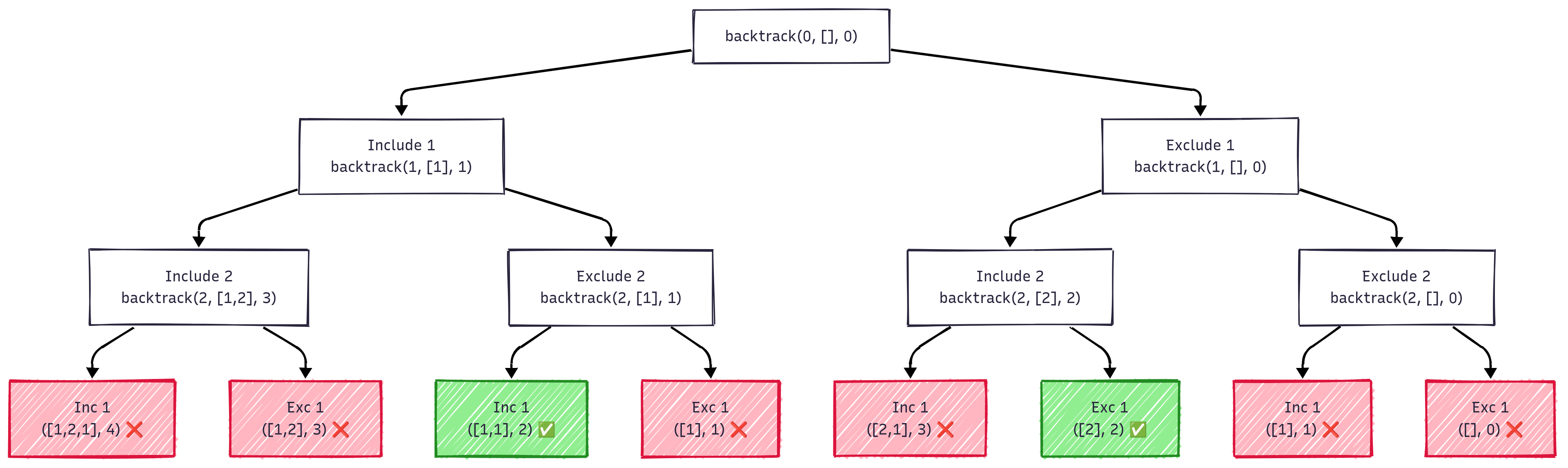
Problem: Given an array and target sum k, find all subsequences that sum to k.
Approach: Use recursion with backtracking. For each element, we have two choices:
- Include the element in current subsequence
- Exclude the element from current subsequence
def print_subsequences_with_sum_k(arr, k):
    def backtrack(index, current_subsequence, current_sum):
        # Base case: processed all elements
        if index == len(arr):
            if current_sum == k:
                print(current_subsequence)
            return

        # Choice 1: Include current element
        current_subsequence.append(arr[index])
        backtrack(index + 1, current_subsequence, current_sum + arr[index])
        current_subsequence.pop()  # backtrack

        # Choice 2: Exclude current element
        backtrack(index + 1, current_subsequence, current_sum)

    backtrack(0, [], 0)

# Example usage
arr = [1, 2, 1]
k = 2
print_subsequences_with_sum_k(arr, k)
# Output: [2], [1, 1]
Recursion Tree for array [1, 2, 1] with k=2:
Key Points:
- Time Complexity: - each element has 2 choices
- Space Complexity: - recursion depth and subsequence storage
- Pattern: Classic "include/exclude" decision tree
- Optimization: Can add pruning if (for positive numbers)
Optimized version with pruning:
def print_subsequences_with_sum_k_optimized(arr, k):
    def backtrack(index, current_subsequence, current_sum):
        # Pruning: if sum exceeds k, no point continuing (for positive arrays)
        if current_sum > k:
            return

        if index == len(arr):
            if current_sum == k:
                print(current_subsequence[:])  # print copy
            return

        # Include current element
        current_subsequence.append(arr[index])
        backtrack(index + 1, current_subsequence, current_sum + arr[index])
        current_subsequence.pop()

        # Exclude current element
        backtrack(index + 1, current_subsequence, current_sum)
Count the Subsequences with Sum k
def count_subsequences_with_sum_k(arr, k):
    def backtrack(index, current_sum):
        if index == len(arr):
            return 1 if current_sum == k else 0
        # Include current element
        count_including = backtrack(index + 1, current_sum + arr[index])
        # Exclude current element
        count_excluding = backtrack(index + 1, current_sum)
        return count_including + count_excluding
    return backtrack(0, 0)
# Example usage
arr = [1, 2, 1]
k = 2
print(count_subsequences_with_sum_k(arr, k))  # Output: 2
Combination of Subsequences with Sum k
To find all combinations of subsequences that sum to k, we can modify our approach to collect valid subsequences instead of just counting them.
def find_combinations_with_sum_k(arr, k):
    def backtrack(index, current_subsequence, current_sum):
        if current_sum == k:
            print(current_subsequence)
            return
        if index == len(arr) or current_sum > k:
            return
        # Include current element
        current_subsequence.append(arr[index])
        backtrack(index + 1, current_subsequence, current_sum + arr[index])
        current_subsequence.pop()
        # Exclude current element
        backtrack(index + 1, current_subsequence, current_sum)
    backtrack(0, [], 0)
# Example usage
arr = [1, 2, 1]
k = 2
find_combinations_with_sum_k(arr, k)
Print all Permutations of a String/Array
def print_permutations(s):
    def backtrack(path, remaining):
        if not remaining or len(path) == len(s):
            print(''.join(path))
            return
        for i in range(len(remaining)):
            path.append(remaining[i])  # Choose
            backtrack(path, remaining[:i] + remaining[i+1:])   # Explore
            path.pop()  # Un-choose
    backtrack([], list(s))
Optimized solution with swapping to avoid extra space:
def print_permutations_optimized(s):
    def backtrack(start):
        if start == len(s) - 1:
            print(''.join(s))
            return
        for i in range(start, len(s)):
            s[start], s[i] = s[i], s[start]  # swap
            backtrack(start + 1)
            s[start], s[i] = s[i], s[start]  # backtrack (swap back)
    s = list(s)
    backtrack(0)
print_permutations_optimized("ABC")
Best Practices
Do:
- ✅ Always define clear base cases first
- ✅ Ensure each recursive call progresses toward the base case
- ✅ Use memoization for overlapping subproblems
- ✅ Consider iterative solutions for simple cases
- ✅ Test with small inputs first
Don't:
- ❌ Forget the base case
- ❌ Create infinite recursion
- ❌ Use recursion for simple iteration tasks
- ❌ Ignore stack overflow possibilities
- ❌ Modify global state without careful consideration
Binary Search
Binary search is a highly efficient algorithm for finding an item from a sorted list of items. It works by repeatedly dividing the search interval in half. If the value of the search key is less than the item in the middle of the interval, the search continues in the lower half, or if it's greater, in the upper half. This process repeats until the value is found or the interval is empty.
def binary_search(arr, target):
    left, right = 0, len(arr) - 1

    while left <= right:
        mid = left + (right - left) // 2

        if arr[mid] == target:
            return mid  # Target found
        elif arr[mid] < target:
            left = mid + 1  # Search in the right half
        else:
            right = mid - 1  # Search in the left half

    return -1  # Target not found
Binary Search Recursively:
def binary_search_recursive(arr, target, left, right):
    if left > right:
        return -1  # Target not found

    mid = left + (right - left) // 2

    if arr[mid] == target:
        return mid  # Target found
    elif arr[mid] < target:
        return binary_search_recursive(arr, target, mid + 1, right)  # Search in the right half
    else:
        return binary_search_recursive(arr, target, left, mid - 1)  # Search in the left half
Time Complexity: O(log n) - Each step reduces the search space by half.
Tree Data Structure
A tree is a hierarchical data structure consisting of nodes, where each node contains a value and references to its child nodes. The topmost node is called the root, and nodes without children are called leaves. Trees are widely used in computer science for various applications, including representing hierarchical data, facilitating fast search operations, and organizing data for efficient access.
Types of Trees
- Binary Tree: Each node has at most two children (left and right).
- Binary Search Tree (BST): A binary tree where the left child's value is less than the parent's value, and the right child's value is greater.
- Full Binary Tree: Every node has either 0 or 2 children.
- Complete Binary Tree: All levels are fully filled except possibly the last, which is filled from left to right.
- Balanced Trees: Trees that maintain a balanced height to ensure efficient operations (e.g., AVL Tree, Red-Black Tree).
- Trie: A tree used for storing a dynamic set of strings, where each node represents a character.
- Heap: A complete binary tree that satisfies the heap property (max-heap or min-heap).
- Segment Tree: A tree used for storing intervals or segments, allowing efficient range queries and updates.
A Tree is typically traversed in two ways:
- Breadth First Traversal (Or Level Order Traversal)
- Depth First Traversals
- Inorder Traversal (Left-Root-Right)
- Preorder Traversal (Root-Left-Right)
- Postorder Traversal (Left-Right-Root)
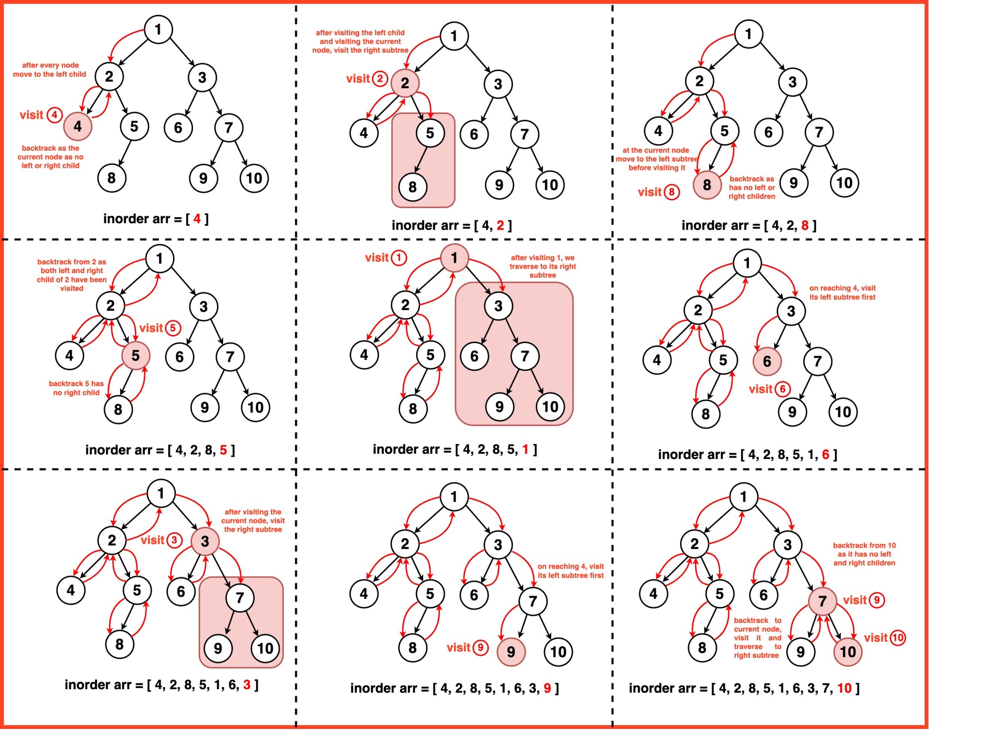
Inorder Traversal of Binary Tree
Inorder traversal visits nodes in the following order: left subtree, root node, right subtree. This traversal method is particularly useful for binary search trees (BSTs) because it retrieves values in sorted order.
class Node:
    def __init__(self, key):
        self.left = None
        self.right = None
        self.val = key

def inorder_traversal(root):
    if root is None:
        return
    inorder_traversal(root.left)
    print(root.val, end=' ')
    inorder_traversal(root.right)

def inorder_traversal_iterative(root):
    stack = []
    current = root

    while stack or current:
        while current:
            stack.append(current)
            current = current.left
        current = stack.pop()
        print(current.val, end=' ')
        current = current.right

# Example usage:
if __name__ == "__main__":
    root = Node(1)
    root.left = Node(2)
    root.right = Node(3)
    root.left.left = Node(4)
    root.left.right = Node(5)

    print("Inorder traversal of binary tree is:")
    inorder_traversal(root)  # Output: 4 2 5 1 3
Postorder Traversal of Binary Tree
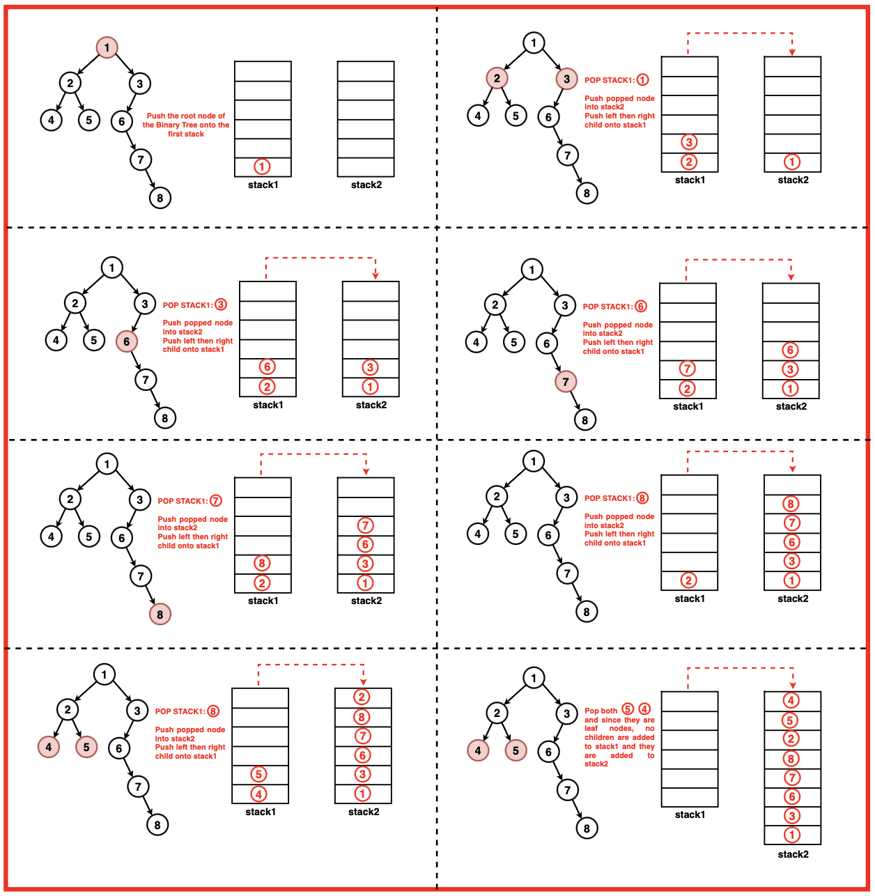
In postorder traversal, the nodes are recursively visited in this order: left subtree, right subtree, and then the root node. This traversal is particularly useful for deleting trees or evaluating postfix expressions.
class Node:
    def __init__(self, key):
        self.left = None
        self.right = None
        self.val = key

def postorder_traversal(root):
    if root is None:
        return
    postorder_traversal(root.left)
    postorder_traversal(root.right)
    print(root.val, end=' ')

def postorder_traversal_iterative(root):
    if root is None:
        return
    stack1 = [root]
    stack2 = []
    while stack1:
        node = stack1.pop()
        stack2.append(node)
        if node.left:
            stack1.append(node.left)
        if node.right:
            stack1.append(node.right)
    while stack2:
        node = stack2.pop()
        print(node.val, end=' ')

# iterative version using one stack
def postorder_traversal_iterative_one_stack(root):
    if root is None:
        return
    stack = []
    current = root
    while stack or current:
        if current:
            stack.append(current)
            current = current.left
        else:
            temp = stack[-1].right
            if temp is None:
                temp = stack.pop()
                print(temp.val, end=' ')
                while stack and temp == stack[-1].right:
                    temp = stack.pop()
                    print(temp.val, end=' ')
            else:
                current = temp

# Example usage:
if __name__ == "__main__":
    root = Node(1)
    root.left = Node(2)
    root.right = Node(3)
    root.left.left = Node(4)
    root.left.right = Node(5)
    print("Postorder traversal of binary tree is:")
postorder_traversal(root) # Output: 4 5 2 3 1Preorder Traversal of Binary Tree
In preorder traversal, the nodes are recursively visited in this order: root node, left subtree, and then right subtree. This traversal is useful for creating a copy of the tree or for prefix expression evaluation.
class Node:
    def __init__(self, key):
        self.left = None
        self.right = None
        self.val = key

def preorder_traversal(root):
    if root is None:
        return
    print(root.val, end=' ')
    preorder_traversal(root.left)
    preorder_traversal(root.right)

def preorder_traversal_iterative(root):
    if root is None:
        return
    stack = [root]
    while stack:
        node = stack.pop()
        print(node.val, end=' ')
        if node.right:
            stack.append(node.right)
        if node.left:
            stack.append(node.left)

# Example usage:
if __name__ == "__main__":
    root = Node(1)
    root.left = Node(2)
    root.right = Node(3)
    root.left.left = Node(4)
    root.left.right = Node(5)
    print("Preorder traversal of binary tree is:")
    preorder_traversal(root)  # Output: 1 2 4 5 3
Height of a Binary Tree
The height of a binary tree is defined as the number of edges on the longest path from the root node to a leaf node. If the tree is empty, the height is -1. If the tree has only one node (the root), the height is 0.
class Node:
    def __init__(self, key):
        self.left = None
        self.right = None
        self.val = key

def height_of_tree_dfs_recursive(root):
    if root is None:
        return -1  # Height of empty tree is -1
    else:
        left_height = height_of_tree_dfs_recursive(root.left)
        right_height = height_of_tree_dfs_recursive(root.right)
        return max(left_height, right_height) + 1

def height_of_tree_bfs_with_depth(root):
    if root is None:
        return -1
    from collections import deque
    queue = deque([(root, 0)])  # (node, current_depth_in_edges)
    max_height = 0
    while queue:
        node, depth = queue.popleft()
        max_height = max(max_height, depth)
        if node.left:
            queue.append((node.left, depth + 1))
        if node.right:
            queue.append((node.right, depth + 1))
    return max_height

def height_of_tree_bfs_level_order(root):
    if root is None:
        return -1
    from collections import deque
    queue = deque([root])
    levels = 0
    while queue:
        for _ in range(len(queue)):
            node = queue.popleft()
            if node.left:
                queue.append(node.left)
            if node.right:
                queue.append(node.right)
        levels += 1
return levels - 1Lower bound and Upper bound in a sorted array
-
Lower Bound: The lower bound of a target value in a sorted array is the index of the first element that is not less than (i.e., greater than or equal to) the target. If all elements are less than the target, it returns the length of the array.
-
Upper Bound: The upper bound of a target value in a sorted array is the index of the first element that is greater than the target. If all elements are less than or equal to the target, it returns the length of the array.
def lower_bound(arr, target):
    left, right = 0, len(arr)
    while left < right:
        mid = left + (right - left) // 2
        if arr[mid] < target:
            left = mid + 1
        else:
            right = mid
    return left

def upper_bound(arr, target):
    left, right = 0, len(arr)
    while left < right:
        mid = left + (right - left) // 2
        if arr[mid] <= target:
            left = mid + 1
        else:
            right = mid
    return left
Segment Tree
A Segment Tree is a binary tree used for storing intervals or segments. It allows querying which of the stored segments contain a given point efficiently. It is particularly useful for answering range queries and performing updates on an array.
class SegmentTree:
    """
    Segment Tree data structure for efficient range queries and updates.
    Supports range sum queries and point updates in O(log n) time.
    """

    class Node:
        def __init__(self, start_interval: int, end_interval: int):
            self.data = 0
            self.start_interval = start_interval
            self.end_interval = end_interval
            self.left = None
            self.right = None

        def __repr__(self):
            return f"Node([{self.start_interval}-{self.end_interval}], data={self.data})"

    def __init__(self, arr: list[int]):
        if not arr:
            raise ValueError("Array cannot be empty")
        self.root = self._construct_tree(arr, 0, len(arr) - 1)

    def _construct_tree(self, arr: list[int], start: int, end: int) -> Node:
        """
        Recursively construct the segment tree.

        Args:
            arr: Input array
            start: Start index of current segment
            end: End index of current segment

        Returns:
            Root node of the constructed subtree
        """
        if start == end:
            # Leaf node
            leaf = self.Node(start, end)
            leaf.data = arr[start]
            return leaf

        # Create new node for current segment
        node = self.Node(start, end)

        # Avoid potential overflow with this mid calculation
        mid = start + (end - start) // 2

        node.left = self._construct_tree(arr, start, mid)
        node.right = self._construct_tree(arr, mid + 1, end)
        node.data = node.left.data + node.right.data

        return node

    def display(self):
        if self.root:
            self._display(self.root)

    def _display(self, node: Node):
        parts = []

        if node.left:
            parts.append(f"Interval=[{node.left.start_interval}-{node.left.end_interval}] and data: {node.left.data} => ")
        else:
            parts.append("No left child => ")

        # Current node
        parts.append(f"Interval=[{node.start_interval}-{node.end_interval}] and data: {node.data}")

        if node.right:
            parts.append(f" <= Interval=[{node.right.start_interval}-{node.right.end_interval}] and data: {node.right.data}")
        else:
            parts.append(" <= No right child")

        print(''.join(parts) + '\n')

        if node.left:
            self._display(node.left)
        if node.right:
            self._display(node.right)

    def query(self, qsi: int, qei: int) -> int:
        """
        Perform range sum query.

        Args:
            qsi: Query start index
            qei: Query end index

        Returns:
            Sum of elements in range [qsi, qei]
        """
        return self._query(self.root, qsi, qei)

    def _query(self, node: Node, qsi: int, qei: int) -> int:
        """
        Recursively perform range query.

        Args:
            node: Current node
            qsi: Query start index
            qei: Query end index

        Returns:
            Sum for the queried range
        """
        # Node completely lies inside query range
        if node.start_interval >= qsi and node.end_interval <= qei:
            return node.data

        # Node completely outside query range
        if node.start_interval > qei or node.end_interval < qsi:
            return 0

        # Partial overlap - query both children
        return self._query(node.left, qsi, qei) + self._query(node.right, qsi, qei)

    def update(self, index: int, value: int):
        """
        Update value at a specific index.

        Args:
            index: Index to update
            value: New value
        """
        self._update(self.root, index, value)

    def _update(self, node: Node, index: int, value: int) -> int:
        """
        Recursively update the value at given index.

        Args:
            node: Current node
            index: Index to update
            value: New value

        Returns:
            Updated data value for current node
        """
        # Check if index lies in current node's range
        if index >= node.start_interval and index <= node.end_interval:
            # Leaf node - update the value
            if index == node.start_interval and index == node.end_interval:
                node.data = value
                return node.data

            # Internal node - update children and recalculate
            left_ans = self._update(node.left, index, value)
            right_ans = self._update(node.right, index, value)
            node.data = left_ans + right_ans
            return node.data

        return node.data

if __name__ == "__main__":
    # Create segment tree
    arr = [1, 3, 5, 7, 9, 11]
    seg_tree = SegmentTree(arr)

    print("Segment Tree Structure:")
    seg_tree.display()

    # Query examples
    print("\n--- Range Queries ---")
    print(f"Sum of range [1, 4]: {seg_tree.query(1, 4)}")  # 3+5+7+9 = 24
    print(f"Sum of range [0, 2]: {seg_tree.query(0, 2)}")  # 1+3+5 = 9

    # Update example
    print("\n--- Update Operation ---")
    print(f"Updating index 2 from {arr[2]} to 10")
    seg_tree.update(2, 10)

    print(f"Sum of range [1, 4] after update: {seg_tree.query(1, 4)}")  # 3+10+7+9 = 29
print(f"Sum of range [0, 2] after update: {seg_tree.query(0, 2)}") # 1+3+10 = 14Greedy Methods and Algorithms
Fundamental Concepts and Definition
What are Greedy Algorithms?
Greedy algorithms are a class of algorithms that solve optimization problems by making locally optimal choices at each step, with the hope of finding a global optimum. The term "greedy" reflects the algorithm's myopic behavior - it grabs the best immediate option without considering future consequences. Programiz
Formal Definition: A greedy algorithm constructs a solution to an optimization problem by iteratively selecting elements that maximize (or minimize) some criterion function at each step , without reconsidering previous choices.
Core Principles The greedy paradigm operates on three fundamental principles:
- Incremental construction: Solutions are built piece by piece
- Irrevocable decisions: Once a choice is made, it cannot be undone
- Local optimization: Each decision optimizes based on current state only
Essential Properties of Greedy Algorithms
Deterministic Nature: Given the same input and selection criteria, a greedy algorithm always produces the same output, making it predictable and analyzable. No Backtracking: Unlike exhaustive search or dynamic programming, greedy algorithms never reconsider or modify previous decisions. This property leads to their efficiency but can also result in suboptimal solutions for certain problems. Simple Decision Rules: Greedy algorithms typically employ straightforward selection criteria such as:
- Maximum or minimum value selection
- Earliest or latest time selection
- Highest ratio or density selection
- Shortest or longest distance selection
Memory Efficiency: Most greedy algorithms require minimal auxiliary space, often or , as they don't need to store multiple solution states or subproblem results.
Algorithmic Characteristics
The general structure of a greedy algorithm follows this pattern:
GREEDY-ALGORITHM(problem_instance):
    solution = ∅
    candidates = INITIALIZE-CANDIDATES(problem_instance)

    while solution is not complete and candidates ≠ ∅:
        x = SELECT-BEST(candidates)
        candidates = candidates - {x}
        if FEASIBLE(solution U {x}):
            solution = solution U {x}

    return solution
The Greedy Choice Property
Definition: A global optimum can be arrived at by making locally optimal (greedy) choices.
Formal Statement: For an optimization problem with objective function and solution space , the greedy choice property holds if:
- partial solution , optimal solution such that contains the greedy choice made from state
Optimal Substructure
Definition: An optimal solution to the problem contains optimal solutions to subproblems.
Mathematical Formulation: If is an optimal solution to problem , and can be decomposed into subproblems , then contains optimal solutions to these subproblems.
Classic Greedy Algorithm Examples
Activity Selection Problem
Problem Statement: Given n activities with start times sᵢ and finish times fᵢ, select the maximum number of non-overlapping activities.
Mathematical Formulation:
- Input: Activities with intervals
- Output: Maximum subset such that ∀ ,
Algorithm:
- Sort activities by increasing finish time.
- Iteratively pick the next activity whose start time ≥ last selected activity's finish time.
- This greedy choice (earliest finishing first) yields an optimal solution.
def select_max_activities(activities):
    """
    activities: list of (start, finish) pairs representing [s, f)
    returns: list of selected (start, finish) pairs forming a maximum-size compatible set
    """
    # 1) Sort by finish time
    activities = sorted(activities, key=lambda x: x[1])

    selected = []
    last_finish = float("-inf")  # allows picking the first interval

    # 2) Greedily select non-overlapping intervals
    for s, f in activities:
        if s >= last_finish:      # [s, f) allows s == last_finish
            selected.append((s, f))
            last_finish = f

    return selected

# Example
if __name__ == "__main__":
    acts = [(1, 4), (3, 5), (0, 6), (5, 7), (8, 9), (5, 9)]
    chosen = select_max_activities(acts)
    print("Selected:", chosen)           # e.g., [(1, 4), (5, 7), (8, 9)]
    print("Maximum count:", len(chosen)) # 3
Time Complexity: for sorting + for selection = Space Complexity: for storing selected activities
Knapsack Problem (Fractional)
Problem Statement: Given n items with weights and values , and knapsack capacity , maximize value while respecting weight constraint. Fractional items allowed.
Mathematical Formulation: Maximize: Subject to: , where
Greedy Strategy
- Sort items by value density in descending order.
- Take whole items while capacity allows; take a fraction of the first item that doesn't fit.
def fractional_knapsack(items, capacity):
    """
    items: list of (value, weight)
    capacity: knapsack capacity
    returns: (max_value, picks) where picks = [(value, weight, fraction_taken), ...]
    """
    # Sort by value density (value/weight), highest first
    items = sorted(items, key=lambda x: x[0] / x[1], reverse=True)

    value = 0.0
    picks = []

    for v, w in items:
        if capacity <= 0:
            break
        if w <= capacity:
            value += v
            picks.append((v, w, 1.0))
            capacity -= w
        else:
            frac = capacity / w
            value += v * frac
            picks.append((v, w, frac))
            break

    return value, picks

# Example
if __name__ == "__main__":
    items = [(60, 10), (100, 20), (120, 30)]
    W = 50
    max_val, taken = fractional_knapsack(items, W)
    print(f"Max value: {max_val:.2f}")        # 240.00
    print("Taken:", taken)                    # [(100, 20, 1.0), (120, 30, 1.0), (60, 10, 0.0)] or similar by density
Time Complexity: for sorting; space .
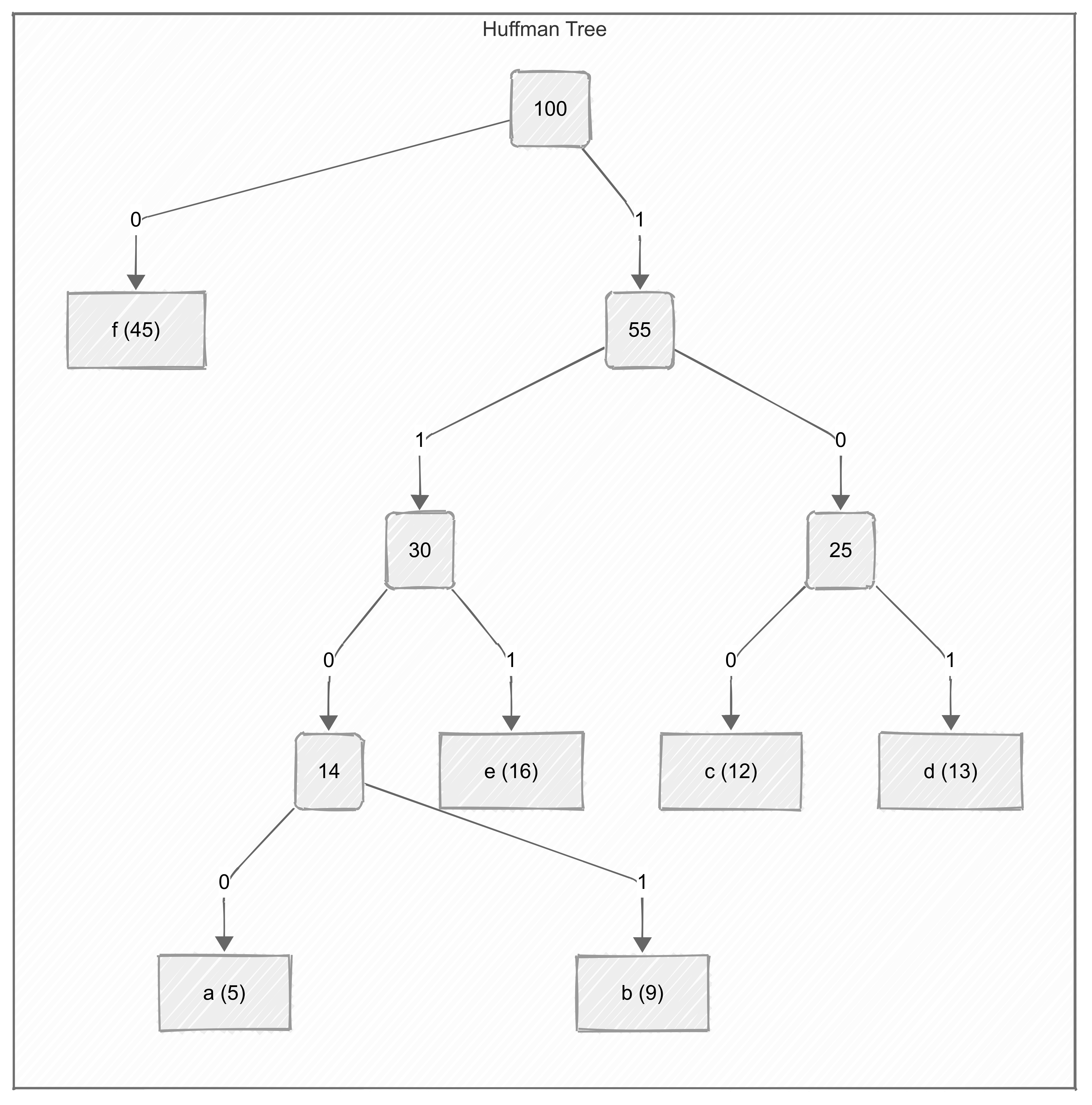
Huffman Coding
Problem Statement: Design optimal prefix-free binary codes for characters based on their frequencies. Mathematical Formulation: Minimize: where is frequency and is code length for character Greedy Strategy:
- Build a min-heap of nodes (characters with frequencies).
- Repeatedly extract two nodes with smallest frequencies, combine them into a new node with summed frequency, and reinsert.
- Continue until one node remains (the root of the Huffman tree).
- Assign binary codes by traversing the tree (left=0, right=1).
Huffman Codes Generated:
| Character | Frequency | Huffman Code | Code Length |
|---|---|---|---|
| f | 45 | 0 | 1 |
| e | 16 | 111 | 3 |
| d | 13 | 101 | 3 |
| c | 12 | 100 | 3 |
| b | 9 | 1101 | 4 |
| a | 5 | 1100 | 4 |
import heapq
from collections import defaultdict
class Node:
    def __init__(self, char, freq):
        self.char = char
        self.freq = freq
        self.left = None
        self.right = None

    def __lt__(self, other):
        return self.freq < other.freq
def huffman_coding(frequencies):
    """
    frequencies: dict of {char: freq}
    returns: dict of {char: huffman_code}
    """
    # Build priority queue (min-heap)
    heap = [Node(char, freq) for char, freq in frequencies.items()]
    heapq.heapify(heap)
    # Build Huffman Tree
    while len(heap) > 1:
        left = heapq.heappop(heap)
        right = heapq.heappop(heap)
        merged = Node(None, left.freq + right.freq)
        merged.left = left
        merged.right = right
        heapq.heappush(heap, merged)
    root = heap[0]
    # Generate codes
    codes = {}
    def generate_codes(node, current_code):
        if node:
            if node.char is not None:
                codes[node.char] = current_code
            generate_codes(node.left, current_code + "0")
            generate_codes(node.right, current_code + "1")
    generate_codes(root, "")
    return codes
# Example
if __name__ == "__main__":
    freqs = {'a': 5, 'b': 9, 'c': 12, 'd': 13, 'e': 16, 'f': 45}
    huff_codes = huffman_coding(freqs)
print("Huffman Codes:", huff_codes)Time Complexity: for building the tree; space for codes.
Minimum Spanning Tree (MST) - Prim's and Kruskal's Algorithms
Problem Statement: Given a connected, undirected graph, find a subset of edges that forms a tree including every vertex, where the total edge weight is minimized.
The algorithm is greedy because at each step, it chooses the minimum weight edge available that maintains the tree property (no cycles).
Mathematical Formulation: Minimize: where ranges over (the set of edges in the spanning tree), and is the weight of edge .
Greedy Strategies:
- Prim's Algorithm: Start from an arbitrary vertex, grow the MST by adding the smallest edge that connects a vertex in the MST to a vertex outside it.
- Initialize a min-heap (priority queue) with the starting vertex and its edges.
- While the min-heap is not empty:
- Extract the minimum weight edge.
- If the edge connects a vertex outside the MST, add it to the MST and include the new vertex.
- Otherwise, discard the edge.
import heapq
def prim_mst(graph, start=0):
    """
    graph: adjacency list {node: [(neighbor, weight), ...]}
    start: starting vertex
    returns: list of edges in the MST and total weight
    """
    mst_edges = []
    total_weight = 0
    visited = set()
    min_heap = [(0, start, None)]  # (weight, current_node, from_node)
    while min_heap:
        weight, u, from_node = heapq.heappop(min_heap)
        if u in visited:
            continue
        visited.add(u)
        total_weight += weight
        if from_node is not None:
            mst_edges.append((from_node, u, weight))
        for v, w in graph[u]:
            if v not in visited:
                heapq.heappush(min_heap, (w, v, u))
    return mst_edges, total_weight
# Example
if __name__ == "__main__":
    graph = {
        0: [(1, 4), (2, 1)],
        1: [(0, 4), (2, 2), (3, 5)],
        2: [(0, 1), (1, 2), (3, 8)],
        3: [(1, 5), (2, 8)]
    }
    mst, weight = prim_mst(graph)
    print("MST Edges:", mst)
    print("Total Weight:", weight)
Time Complexity: using a priority queue; space for visited set and heap.
- Kruskal's Algorithm: Sort all edges by weight, and add them one by one to the MST, skipping those that would form a cycle (using Union-Find to detect cycles).
- Sort edges by weight.
- Initialize a Union-Find structure to track connected components.
- Iterate through sorted edges:
- If the edge connects two different components, add it to the MST and union the components
class UnionFind:
    def __init__(self, size):
        self.parent = list(range(size))
        self.rank = [1] * size

    def find(self, u):
        if self.parent[u] != u:
            self.parent[u] = self.find(self.parent[u])
        return self.parent[u]

    def union(self, u, v):
        root_u = self.find(u)
        root_v = self.find(v)
        if root_u != root_v:
            if self.rank[root_u] > self.rank[root_v]:
                self.parent[root_v] = root_u
            elif self.rank[root_u] < self.rank[root_v]:
                self.parent[root_u] = root_v
            else:
                self.parent[root_v] = root_u
                self.rank[root_u] += 1

def kruskal_mst(edges, num_vertices):
    """
    edges: list of (weight, u, v)
    num_vertices: number of vertices in the graph
    returns: list of edges in the MST and total weight
    """
    edges.sort()  # Sort edges by weight
    uf = UnionFind(num_vertices)
    mst_edges = []
    total_weight = 0
    for weight, u, v in edges:
        if uf.find(u) != uf.find(v):
            uf.union(u, v)
            mst_edges.append((u, v, weight))
            total_weight += weight
    return mst_edges, total_weight
# Example
if __name__ == "__main__":
    edges = [
        (4, 0, 1), (1, 0, 2), (2, 1, 2),
        (5, 1, 3), (8, 2, 3)
    ]
    num_vertices = 4
    mst, weight = kruskal_mst(edges, num_vertices)
    print("MST Edges:", mst)
print("Total Weight:", weight)Dynamic Programming
What is Dynamic Programming? Dynamic Programming is a method for solving complex problems by breaking them down into simpler subproblems and storing the results of these subproblems to avoid redundant computations. It is particularly effective for optimization problems where the solution can be constructed from solutions to smaller subproblems. Formal Definition: A problem exhibits optimal substructure if an optimal solution to the problem contains optimal solutions to its subproblems. It exhibits overlapping subproblems if the same subproblems are solved multiple times during the computation of the overall solution.
Core Principles The dynamic programming paradigm operates on three fundamental principles:
-
Optimal Substructure: The optimal solution to a problem can be constructed from optimal solutions to its subproblems.
-
Overlapping Subproblems: The problem can be broken down into subproblems that
are reused multiple times.
-
Memoization or Tabulation: Store the results of subproblems to avoid redundant computations.
Essential Properties of Dynamic Programming
Deterministic Nature: Given the same input, a dynamic programming algorithm will always produce the same output, making it predictable and analyzable. Optimal Substructure: If a problem can be divided into subproblems, and the optimal solution to the overall problem can be constructed from the optimal solutions of its subproblems, then the problem has optimal substructure. This property is crucial for the applicability of dynamic programming. Overlapping Subproblems: If a problem can be broken down into subproblems that are solved multiple times, then the problem has overlapping subproblems. This property allows dynamic programming to store the results of these subproblems and reuse them, significantly improving efficiency. Memory Efficiency: Dynamic programming algorithms often require additional memory to store the results of subproblems, which can lead to increased space complexity. However, techniques such as space optimization can be employed to reduce memory usage in certain cases.
Classic Dynamic Programming Examples
Fibonacci Sequence
Problem Statement: Compute the n-th Fibonacci number, where each number is the sum of the two preceding ones, starting from 0 and 1. Mathematical Formulation:
- Base Cases:
- Recurrence Relation: for
# Recursive with Memoization
def fibonacci_memo(n, memo={}):
    if n in memo:
        return memo[n]
    if n <= 1:
        return n
    memo[n] = fibonacci_memo(n-1, memo) + fibonacci_memo(n-2, memo)
    return memo[n]

# Iterative with Tabulation
def fibonacci_tab(n):
    if n <= 1:
        return n
    fib = [0] * (n + 1)
    fib[1] = 1
    for i in range(2, n + 1):
        fib[i] = fib[i - 1] + fib[i - 2]
    return fib[n]
# Space Optimized Iterative
def fibonacci_optimized(n):
    if n <= 1:
        return n
    a, b = 0, 1
    for _ in range(2, n + 1):
        a, b = b, a + b
    return b
# Example
if __name__ == "__main__":
    n = 10
    print(f"Fibonacci({n}) with memoization:", fibonacci_memo(n))
    print(f"Fibonacci({n}) with tabulation:", fibonacci_tab(n))
    print(f"Fibonacci({n}) optimized:", fibonacci_optimized(n))
0/1 Knapsack Problem
Problem Statement: Given weights and values of items, put these items in a knapsack of capacity to get the maximum total value in the knapsack. Each item can be included or excluded .
Mathematical Formulation:
- Let be the value and be the weight of item
- Let be the maximum value that can be attained with a knapsack capacity using the first items.
- Recurrence Relation:
- for all
- for all
- if
- if
def knapsack_01(weights, values, W):
    n = len(values)
    dp = [[0 for _ in range(W + 1)] for _ in range(n + 1)]

    for i in range(1, n + 1):
        for w in range(W + 1):
            if weights[i - 1] <= w:
                dp[i][w] = max(dp[i - 1][w], values[i - 1] + dp[i - 1][w - weights[i - 1]])
            else:
                dp[i][w] = dp[i - 1][w]

    return dp[n][W]
# Example
if __name__ == "__main__":
    weights = [3, 4, 6, 5]
    values = [2, 3, 1, 4]
    W = 8
    print("Maximum value in Knapsack =", knapsack_01(weights, values, W))
    # Output: 6
DP table (rows = items added, columns = capacity 0-8):
| items\capacity | 0 | 1 | 2 | 3 | 4 | 5 | 6 | 7 | 8 |
|---|---|---|---|---|---|---|---|---|---|
| 0 (0,0) | 0 | 0 | 0 | 0 | 0 | 0 | 0 | 0 | 0 |
| 1 (3,2) | 0 | 0 | 0 | 2 | 2 | 2 | 2 | 2 | 2 |
| 2 (4,3) | 0 | 0 | 0 | 2 | 3 | 3 | 3 | 5 | 5 |
| 3 (5,4) | 0 | 0 | 0 | 2 | 3 | 4 | 4 | 5 | 6 |
| 4 (6,1) | 0 | 0 | 0 | 2 | 3 | 4 | 4 | 5 | 6 |
Longest Common Subsequence (LCS)
Problem Statement: Given two sequences, find the length of the longest subsequence present in both of them. A subsequence is a sequence that appears in the same relative order but not necessarily contiguous.
Mathematical Formulation:
- Let and
- Let be the length of LCS of and
- Recurrence Relation:
- for all
- for all
- if
- if
def lcs(X, Y):
    m = len(X)
    n = len(Y)
    dp = [[0] * (n + 1) for _ in range(m + 1)]
    for i in range(1, m + 1):
        for j in range(1, n + 1):
            if X[i - 1] == Y[j - 1]:
                dp[i][j] = dp[i - 1][j - 1] + 1
            else:
                dp[i][j] = max(dp[i - 1][j], dp[i][j - 1])
    return dp[m][n]
# Example
if __name__ == "__main__":
    X = "AGGTAB"
    Y = "GXTXAYB"
    print("Length of LCS is", lcs(X, Y))  # Output: 4
DP table (rows = chars of X, columns = chars of Y):
| 0 | 1 (G) | 2 (X) | 3 (T) | 4 (X) | 5 (A) | 6 (Y) | 7 (B) | |
|---|---|---|---|---|---|---|---|---|
| 0 | 0 | 0 | 0 | 0 | 0 | 0 | 0 | 0 |
| 1 (A) | 0 | 0 | 0 | 0 | 0 | 1 | 1 | 1 |
| 2 (G) | 0 | 1 | 1 | 1 | 1 | 1 | 1 | 1 |
| 3 (G) | 0 | 1 | 1 | 1 | 1 | 1 | 1 | 1 |
| 4 (T) | 0 | 1 | 1 | 2 | 2 | 2 | 2 | 2 |
| 5 (A) | 0 | 1 | 1 | 2 | 2 | 3 | 3 | 3 |
| 6 (B) | 0 | 1 | 1 | 2 | 2 | 3 | 3 | 4 |
Time Complexity: where and are the lengths of the two sequences. Space Complexity: for the DP table; can be optimized to by storing only the current and previous rows.
Edit Distance (Levenshtein Distance)
Problem Statement: Given two strings, find the minimum number of operations (insertions, deletions, substitutions) required to convert one string into the other.
Mathematical Formulation:
- Let and
- Let be the edit distance between and
- Recurrence Relation:
- for all (all insertions)
- for all
- if
- if
def edit_distance(X, Y):
    m = len(X)
    n = len(Y)
    dp = [[0] * (n + 1) for _ in range(m + 1)]
    for i in range(m + 1):
        for j in range(n + 1):
            if i == 0:
                dp[i][j] = j  # Insert all j characters
            elif j == 0:
                dp[i][j] = i  # Remove all i characters
            elif X[i - 1] == Y[j - 1]:
                dp[i][j] = dp[i - 1][j - 1]
            else:
                dp[i][j] = 1 + min(dp[i - 1][j], dp[i][j - 1], dp[i - 1][j - 1])
    return dp[m][n]
# Example
if __name__ == "__main__":
    X = "kitten"
    Y = "sitting"
    print("Edit Distance is", edit_distance(X, Y))  # Output: 3
Time Complexity: where and are the lengths of the two strings. Space Complexity: for the DP table; can be optimized to by storing only the current and previous rows.
Longest Increasing Subsequence (LIS)
Given an integer array nums, return the length of the longest strictly increasing subsequence.
Recursive Solution:
class Solution:
    def lengthOfLIS(self, nums: List[int]) -> int:
        n = len(nums)
        return self.LIS(0, -1, nums, n)

    def lengthOfLIS(self, nums: List[int]) -> int:
        n = len(nums)
        dp = [[-1] * (n + 1) for _ in range(n)]
        return self.LIS_DP(0, -1, nums, n, dp)

    def LIS(self, int index, int prev_index, int[] nums, int n) -> int:
        if index == n:
            return 0
        take = 0
        if prev_index == -1 or nums[index] > nums[prev_index]:
            take = 1 + self.LIS(index + 1, index, nums, n)
        not_take = self.LIS(index + 1, prev_index, nums, n)
        return max(take, not_take)

    def LIS_DP(self, index, prev_index, nums, n, dp) -> int:
        if index == n:
            return 0
        if dp[index][prev_index] != -1:
            return dp[index][prev_index]
        take = 0
        if prev_index == -1 or nums[index] > nums[prev_index]:
            take = 1 + self.LIS_DP(index + 1, index, nums, n, dp)
        not_take = self.LIS_DP(index + 1, prev_index, nums, n, dp)
        dp[index][prev_index] = max(take, not_take)
        return dp[index][prev_index]
Mathematical Formulation:
- Let
- Let be the length of the longest increasing subsequence ending at index
- Recurrence Relation:
- for all and
Tabular Solution:
def lis(A):
    n = len(A)
    dp = [1] * n
    for i in range(1, n):
        for j in range(i):
            if A[i] > A[j]:
                dp[i] = max(dp[i], dp[j] + 1)
    return max(dp)
# Example
if __name__ == "__main__":
    A = [10, 9, 2, 5, 3, 7, 101, 18]
    print("Length of LIS is", lis(A))  # Output: 4
DP table (rows = index, columns = length of LIS):
| 0(10) | 1(9) | 2(2) | 3(5) | 4(3) | 5(7) | 6(101) | 7(18) | |
|---|---|---|---|---|---|---|---|---|
| 0 (10) | 1 | 1 | 1 | 1 | 1 | 1 | 1 | 1 |
| 1 (9) | 1 | 1 | 1 | 1 | 1 | 1 | 1 | 1 |
| 2 (2) | 1 | 1 | 1 | 1 | 1 | 1 | 1 | 1 |
| 3 (5) | 1 | 1 | 1 | 2 | 2 | 2 | 2 | 2 |
| 4 (3) | 1 | 1 | 1 | 2 | 2 | 2 | 2 | 2 |
| 5 (7) | 1 | 1 | 1 | 2 | 2 | 3 | 3 | 3 |
| 6 (101) | 1 | 1 | 1 | 2 | 2 | 3 | 4 | 4 |
| 7 (18) | 1 | 1 | 1 | 2 | 2 | 3 | 4 | 4 |
Time Complexity: where is the length of the array. Space Complexity: for the DP table.
Graph Data Structures and Algorithms
Graph Data Structures
Graphs are abstract data types that consist of a set of nodes (or vertices) and a set of edges connecting pairs of nodes. They are used to model relationships and connections in various domains, such as social networks, transportation systems, and communication networks.
Graph Representations
-
Adjacency Matrix: A 2D array where the cell at row
iand columnjindicates the presence (and possibly weight) of an edge between vertexiand vertexj. This representation is efficient for dense graphs but can be space-inefficient for sparse graphs.- Space Complexity: where is the number of vertices.
- Time Complexity: for edge look-up, for iterating over neighbors.
class GraphAdjMatrix: def __init__(self, vertices): self.V = vertices self.adj_matrix = [[0] * vertices for _ in range(vertices)] def add_edge(self, u, v, weight=1): self.adj_matrix[u][v] = weight self.adj_matrix[v][u] = weight # For undirected graph def remove_edge(self, u, v): self.adj_matrix[u][v] = 0 self.adj_matrix[v][u] = 0 def display(self): for row in self.adj_matrix: print(row) -
Adjacency List: A list where each vertex has a list of its adjacent vertices (and possibly edge weights). This representation is more space-efficient for sparse graphs.
- Space Complexity: where is the number of edges.
- Time Complexity: for edge look-up, for iterating over neighbors.
class GraphAdjList:
     def __init__(self):
          self.adj_list = {}

     def add_edge(self, u, v, weight=1):
          if u not in self.adj_list:
            self.adj_list[u] = []
          if v not in self.adj_list:
            self.adj_list[v] = []
          self.adj_list[u].append((v, weight))
          self.adj_list[v].append((u, weight))  # For undirected graph

     def remove_edge(self, u, v):
          if u in self.adj_list:
            self.adj_list[u] = [pair for pair in self.adj_list[u] if pair[0] != v]
          if v in self.adj_list:
            self.adj_list[v] = [pair for pair in self.adj_list[v] if pair[0] != u]

     def display(self):
          for key in self.adj_list:
            print(f"{key}: {self.adj_list[key]}")
Breadth First Search (BFS)
Given an undirected graph, return a vector of all nodes by traversing the graph using breadth-first search (BFS).
from collections import deque

def BFS(graph, start):
    visited = set()
    queue = deque([start])
    visited.add(start)
    while queue:
        node = queue.popleft()
        print(node)
        for neighbor in graph[node]:
            if neighbor not in visited:
                visited.add(neighbor)
                queue.append(neighbor)

graph = {
    'A': ['B', 'C'],
    'B': ['A', 'D'],
    'C': ['A', 'D'],
    'D': ['B', 'C']
}

BFS(graph, 'A')
Depth First Search (DFS)
Given an undirected graph, return a vector of all nodes by traversing the graph using depth-first search (DFS).
from collections import deque

def DFS(graph, start):
    visited = set()
    stack = deque([start])
    visited.add(start)
    while stack:
        node = stack.pop()
        print(node)
        for neighbor in graph[node]:
            if neighbor not in visited:
                visited.add(neighbor)
                stack.append(neighbor)

visited = set()
def DFS_recursive(graph, start, visited):
    visited.add(start)
    print(start)
    for neighbor in graph[start]:
        if neighbor not in visited:
            DFS_recursive(graph, neighbor, visited)


graph = {
    'A': ['B', 'C'],
    'B': ['A', 'D'],
    'C': ['A', 'D'],
    'D': ['B', 'C']
}

DFS(graph, 'A')

DFS_recursive(graph, 'A', visited)
Disjoint Set | Union by Rank | Union by Size | Path Compression
disjoint set is a data structure that stores a collection of disjoint sets.
- Union by Rank: Union the smaller tree under the larger tree.
- Union by Size: Union the smaller tree under the larger tree.
- Path Compression: Compress the path from the root to the node.
Disjoint Set Union by Rank:
class DisjointSet:
    def __init__(self, size):
        self.parent = list(range(size))
        self.rank = [1] * size

    def find(self, u):
        if self.parent[u] != u:
            self.parent[u] = self.find(self.parent[u])
        return self.parent[u]

    def union(self, u, v):
        parent_u = self.find(u)
        parent_v = self.find(v)
        if parent_u != parent_v:
            if self.rank[parent_u] > self.rank[parent_v]:
                self.parent[parent_v] = parent_u # smaller tree under larger tree
            elif self.rank[parent_u] < self.rank[parent_v]:
                self.parent[parent_u] = parent_v # smaller tree under larger tree
            else: # rank is equal, so we can choose any tree as the parent
                self.parent[parent_v] = parent_u
                self.rank[parent_u] += 1 # increment the rank of the parent

    def is_connected(self, u, v):
        return self.find(u) == self.find(v)

    def get_num_sets(self):
        return sum(1 for i in range(len(self.parent)) if self.parent[i] == i)

# Example
if __name__ == "__main__":
    disjoint_set = DisjointSet(5)
    disjoint_set.union(0, 1)
    disjoint_set.union(1, 2)
    disjoint_set.union(2, 3)
    disjoint_set.union(3, 4)
    print(disjoint_set.is_connected(0, 4))
    print(disjoint_set.get_num_sets())
    print(disjoint_set.parent)
    print(disjoint_set.rank)
Disjoint Set Union by Size:
class DisjointSet:
    def __init__(self, size):
        self.parent = list(range(size))
        self.size = [1] * size

    def find(self, u):
        if self.parent[u] != u:
            self.parent[u] = self.find(self.parent[u])
        return self.parent[u]

    def union(self, u, v):
        parent_u = self.find(u)
        parent_v = self.find(v)
        if parent_u != parent_v:
            if self.size[parent_u] > self.size[parent_v]:
                self.parent[parent_v] = parent_u
                self.size[parent_u] += self.size[parent_v]
            else:
                self.parent[parent_u] = parent_v
                self.size[parent_v] += self.size[parent_u]

    def is_connected(self, u, v):
        return self.find(u) == self.find(v)

    def get_num_sets(self):
        return sum(1 for i in range(len(self.parent)) if self.parent[i] == i)

    def get_size(self, u):
        return self.size[self.find(u)]

# Example
if __name__ == "__main__":
    disjoint_set = DisjointSet(5)
    disjoint_set.union(0, 1)
    disjoint_set.union(1, 2)
    disjoint_set.union(2, 3)
    disjoint_set.union(3, 4)
    print(disjoint_set.is_connected(0, 4))
    print(disjoint_set.get_num_sets())
    print(disjoint_set.parent)
    print(disjoint_set.size)
    print(disjoint_set.find(0))
    print(disjoint_set.find(1))
    print(disjoint_set.find(2))
    print(disjoint_set.find(3))
print(disjoint_set.find(4))Example question on DSU:
Given N products, you do not know in advance how many categories exist, nor do you have an explicit mapping of products to categories. Instead, you are provided with a list of pairs of product IDs, where each pair means that the two products belong to the same category.
Your goal is to process this list of ID pairs and group the products into categories such that:
- Any products that are connected, either directly or through a chain of pairs, end up in the same category.
- Each category contains all products that are transitively associated via the relationships in the pairs.
Example: Input pairs: (1, 5), (7, 2), (3, 4), (4, 8), (6, 3), (5, 2)
Explanation:
- (1, 5) groups 1 and 5 together.
- (7, 2), (5, 2): 1, 5, 2, and 7 end up in one group since they are interconnected.
- (3, 4), (4, 8), (6, 3): 3, 4, 8, and 6 all link together to form a different group.
Output: Two groups: (1, 2, 5, 7) and (3, 4, 6, 8)
To clarify:
- Any two products are in the same group if they are linked through any sequence of pairs.
- The resulting groups do not overlap.
Write a function that takes a list of product ID pairs as input and returns a list of sets (or lists) of IDs, where each set represents one category.
class UnionFind:
    def __init__(self):
        self.parent = {}
        self.rank = {}

    def find(self, x):
        if x not in self.parent:
            self.parent[x] = x
            self.rank[x] = 0
        if self.parent[x] != x:
            self.parent[x] = self.find(self.parent[x])  # path compression
        return self.parent[x]

    def union(self, x, y):
        rx, ry = self.find(x), self.find(y)
        if rx == ry:
            return
        # union by rank
        if self.rank[rx] < self.rank[ry]:
            rx, ry = ry, rx
        self.parent[ry] = rx
        if self.rank[rx] == self.rank[ry]:
            self.rank[rx] += 1


def group_products(pairs):
    uf = UnionFind()
    for a, b in pairs:
        uf.union(a, b)

    groups = {}
    for node in uf.parent:
        root = uf.find(node)
        groups.setdefault(root, []).append(node)

    return tuple(tuple(sorted(g)) for g in groups.values())


# Test cases
pairs1 = ((1,2), (2,5), (3,4), (4,6), (6,8), (5,7), (5,2), (5,2))
print(group_products(pairs1))
# Output: ((1, 2, 5, 7), (3, 4, 6, 8))

pairs2 = ((1,2), (2,5), (3,4), (4,6), (6,8), (5,7), (5,2), (3,1))
print(group_products(pairs2))
# Output: ((1, 2, 3, 4, 5, 6, 7, 8))Time Complexity: for the sort operation, for the Union-Find operations, where is the number of product pairs and is the inverse Ackermann function. Space Complexity: for the Union-Find data structure.
Topological Sort
Topological Sort is a linear ordering of the vertices of a directed graph such that for every directed edge uv from vertex u to vertex v, u comes before v in the ordering. It is only possible for Directed Acyclic Graphs (DAGs).
Mathematical Formulation: A topological sort of a directed graph is a linear ordering of its vertices such that for every directed edge uv from vertex u to vertex v, u comes before v in the ordering.
Algorithm:
- Compute in-degree for each vertex.
- Initialize a queue and enqueue all vertices with in-degree 0.
- While the queue is not empty:
- Dequeue a vertex.
- Add it to the topological order.
- For each neighbor of the vertex, reduce its in-degree by 1.
- If a neighbor's in-degree becomes 0, enqueue it.
Time Complexity: where is the number of vertices and is the number of edges. Space Complexity: for the queue and the topological order.
def topological_sort(graph):
    in_degree = {u: 0 for u in graph}
    for u in graph:
        for v in graph[u]:
            in_degree[v] += 1
    queue = [u for u in graph if in_degree[u] == 0]
    topological_order = []
    while queue:
        u = queue.pop(0)
        topological_order.append(u)
        for v in graph[u]:
            in_degree[v] -= 1
            if in_degree[v] == 0:
                queue.append(v)
    return topological_order
Implementation of Topological Sort using DFS:
def topological_sort_dfs(graph):
    visited = set()
    stack = []
    for u in graph:
        if u not in visited:
            topological_sort_dfs_helper(graph, u, visited, stack)
    return stack[::-1]

def topological_sort_dfs_helper(graph, u, visited, stack):
    visited.add(u)
    for v in graph[u]:
        if v not in visited:
            topological_sort_dfs_helper(graph, v, visited, stack)
    stack.appedn(u)

graph = {
    'A': ['B', 'C'],
    'B': ['D'],
    'C': ['D'],
    'D': []
}
print(topological_sort_dfs(graph))
# Output: ['A', 'C', 'B', 'D']
Bipartite Graph
A bipartite graph is a graph that can be colored using two colors such that no two adjacent nodes have the same color.
Algorithm:
- Color the source node with one color.
- For each neighbor of the source node, color it with the opposite color.
- Repeat the process for each neighbor of the source node.
- If a neighbor has the same color as the source node, return False.
- If all neighbors have been colored, return True.
Using BFS to check if a graph is bipartite:
def is_bipartite(graph):
    # graph: adjacency list, nodes 0..n-1
    n = len(graph)
    color = [-1] * n  # -1 = unvisited, 0 and 1 = two colors

    for start in range(n):
        if color[start] != -1:
            continue
        q = [start]
        color[start] = 0

        while q:
            u = q.pop(0)
            for v in graph[u]:
                if color[v] == -1:
                    color[v] = 1 - color[u]
                    q.append(v)
                elif color[v] == color[u]:
                    return False
    return True
Time Complexity:
- V: We touch each vertex at most once (enqueue and assign a color).
- E: We look at each edge once when we iterate over each vertex's neighbors.
Detect cycle in a directed graph using DFS
To detect cycles in a directed graph using DFS, the key idea is to track not only which nodes we've visited, but also which nodes are currently being explored in our current recursive call stack (the "path" we're traversing). If, while exploring from a node, we run into another node that's already on our current path, we've found a cycle.
Here's how it works, step by step:
-
Use two data structures:
- One to remember which nodes we've ever visited.
- Another to keep track of nodes that are part of the current DFS chain (the recursion stack or path).
-
For every unvisited node in the graph, start a DFS.
- When visiting a node, mark it as visited and add it to the current path stack.
- Then, for each of this node's neighbors:
- If a neighbor hasn't been visited yet, recursively DFS into it.
- If a neighbor is already on the current path, we've returned to a node we're still exploring, so a cycle exists.
- After checking all neighbors, remove the current node from the path stack (since its exploration is finished).
-
If DFS finishes from all nodes without ever finding a node already on the current path, the graph has no cycles (it's a Directed Acyclic Graph).
This approach works efficiently because it checks for cycles as we go, directly within the traversal, and doesn't need to generate a topological order or rely on in-degrees.
In summary:
- Mark nodes as you visit them and track the current traversal path.
- If you hit a node that's already on your path while recursing, you found a cycle.
- Backtrack (remove nodes from the path) as you unwind recursion.
- No cycles found after full search? The graph is acyclic.
def has_cycle(graph):
    visited = set()
    path = set()
    for node in graph:
        if node not in visited:
            if has_cycle_helper(graph, node, visited, path):
                return True
    return False

def has_cycle_helper(graph, node, visited, path):
    visited.add(node)
    path.add(node)
    for neighbor in graph[node]:
        if neighbor not in visited:
            if has_cycle_helper(graph, neighbor, visited, path):
                return True
        if neighbor in path:           # ← ADD THIS: cycle = back edge to ancestor
            return True
    path.remove(node)
    return False
Kahn's Algorithm
Kahn's Algorithm is a topological sort algorithm that is used to sort the vertices of a directed graph in a linear order such that for every directed edge uv from vertex u to vertex v, u comes before v in the ordering.
Algorithm:
- Compute in-degree for each vertex.
- Initialize a queue and enqueue all vertices with in-degree 0.
- While the queue is not empty:
- Dequeue a vertex.
- Add it to the topological order.
- For each neighbor of the vertex, reduce its in-degree by 1.
- If a neighbor's in-degree becomes 0, enqueue it.
from collections import deque

def kahn_topological_sort(graph: dict[int, list[int]], num_vertices: int) -> list[int]:
    # Step 1: Compute in-degree for each vertex
    in_degree = [0] * num_vertices
    for u in graph:
        for v in graph[u]:
            in_degree[v] += 1

    # Step 2: Initialize queue with vertices having in-degree 0
    queue = deque(v for v in range(num_vertices) if in_degree[v] == 0)
    topo_order = []

    # Step 3: Process queue
    while queue:
        u = queue.popleft()
        topo_order.append(u)

        for v in graph.get(u, []):
            in_degree[v] -= 1
            if in_degree[v] == 0:
                queue.append(v)

    # If topo_order has fewer than num_vertices elements, there's a cycle
    if len(topo_order) != num_vertices:
        return []  # Cycle detected

    return topo_order

# Example usage:
# Graph: 0 -> 1, 0 -> 2, 1 -> 3, 2 -> 3 (4 vertices)
graph = {
    0: [1, 2],
    1: [3],
    2: [3],
}
print(kahn_topological_sort(graph, 4))  # [0, 1, 2, 3] or [0, 2, 1, 3]
Time Complexity: where is the number of vertices and is the number of edges. Space Complexity: for the queue and the topological order.
Some important Alogorithms
Kadane's Algorithm : Maximum Subarray Sum in an Array
The intuition behind Kadane's Algorithm is to iterate through the array while maintaining a running sum of the current subarray. If the running sum becomes negative, it is reset to zero. The maximum sum encountered during the iteration is the result.
Steps:
- Iterate over the array with a loop (index i).
- Add each element to a running sum and update the maximum sum when the running sum is larger.
- If the running sum becomes negative, reset it to 0 since continuing from a negative sum cannot improve the result.
def maxSubarraySum(arr, n):
    maximum_sum = float('-inf')
    sum = 0
    start = 0
    subarrayStartIndex, subarrayEndIndex = -1, -1
    for i in range(n):
        if sum == 0:
            start = i
        sum += arr[i]
        if sum > maximum_sum:
            maximum_sum = sum
            subarrayStartIndex = start
            subarrayEndIndex = i
        # If sum < 0: discard the sum calculated
        if sum < 0:
            sum = 0

    print("The subarray is: [", end="")
    for i in range(subarrayStartIndex, subarrayEndIndex + 1):
        print(arr[i], end=" ")
    print("]")
    return maximum_sum

arr = [-2, 1, -3, 4, -1, 2, 1, -5, 4]
n = len(arr)
maxSum = maxSubarraySum(arr, n)
print("The maximum subarray sum is:", maxSum)
Dijkstra's Algorithm
Dijkstra's Algorithm is a shortest path algorithm that is used to find the shortest path between two nodes in a graph.
Algorithm:
- Initialize a distance array with infinity for all nodes except the source node.
- Initialize a priority queue and enqueue the source node with distance 0.
- While the priority queue is not empty:
- Dequeue a node.
- For each neighbor of the node, update the distance if the new distance is smaller.
- If a neighbor's distance is updated, enqueue it with the new distance.
import heapq

def dijkstra(g, n, s):
    """
    Runs Dijkstra's algorithm and returns an array that contains
    the shortest distance to every node from the start node s.

    :param g: Adjacency list where g[i] is a list of (to_node, cost) tuples
    :param n: The number of nodes in the graph
    :param s: The index of the starting node (0 <= s < n)
    :return: List of shortest distances from s to all other nodes
    """
    vis = [False] * n
    dist = [float('inf')] * n
    dist[s] = 0
    pq = []
    heapq.heappush(pq, (0, s))

    while pq:
        minValue, index = heapq.heappop(pq)
        vis[index] = True
        # This handles cases where a node was added to the PQ multiple times
        if dist[index] < minValue:
            continue
        for edge_to, edge_cost in g[index]:
            if vis[edge_to]:
                continue
            new_dist = dist[index] + edge_cost
            if new_dist < dist[edge_to]:
                dist[edge_to] = new_dist
                heapq.heappush(pq, (new_dist, edge_to))
    return dist

if __name__ == "__main__":
    # Graph represented as an adjacency list: g[from] = [(to, cost), ...]
    num_nodes = 5
    graph = [[] for _ in range(num_nodes)]
    # Adding edges: (from, to, cost)
    edges = [
        (0, 1, 4), (0, 2, 1),
        (2, 1, 2), (2, 3, 5),
        (1, 3, 1), (3, 4, 3)
    ]

    for u, v, w in edges:
        graph[u].append((v, w))

    start_node = 0
    distances = dijkstra(graph, num_nodes, start_node)

    print(f"Shortest distances from node {start_node}:")
    for i, d in enumerate(distances):
print(f"To node {i}: {d}")Dijkstra's Algorithm with Path Reconstruction
import heapq

def dijkstra(g, n, s):
    """
    Runs Dijkstra's algorithm and returns distances and previous nodes.

    :param g: Adjacency list where g[i] is a list of (neighbor, cost) tuples
    :param n: Number of nodes in the graph
    :param s: Index of the starting node (0 <= s < n)
    :return: A tuple (dist, prev)
    """
    vis = [False] * n
    prev = [None] * n
    dist = [float('inf')] * n
    dist[s] = 0
    pq = []

    heapq.heappush(pq, (0, s))

    while pq:
        min_value, index = heapq.heappop(pq)
        vis[index] = True
        if dist[index] < min_value:
            continue
        for neighbor, cost in g[index]:
            if vis[neighbor]:
                continue
            new_dist = dist[index] + cost
            if new_dist < dist[neighbor]:
                prev[neighbor] = index
                dist[neighbor] = new_dist
                heapq.heappush(pq, (new_dist, neighbor))
    return dist, prev

num_nodes = 4
adj_list = [
    [(1, 4), (2, 1)], # Edges from node 0
    [(3, 1)],         # Edges from node 1
    [(1, 2), (3, 5)], # Edges from node 2
    []                # Edges from node 3
]

start_node = 0
distances, previous_nodes = dijkstra(adj_list, num_nodes, start_node)

print(f"Distances from node {start_node}: {distances}")
print(f"Previous nodes: {previous_nodes}")